


Abstract
We train convolutional neural networks to predict whether or not a set of measurements is informationally complete to uniquely reconstruct any given quantum state with no prior information. In addition, we perform fidelity benchmarking based on this measurement set without explicitly carrying out state tomography. The networks are trained to recognize the fidelity and a reliable measure for informational completeness. By gradually accumulating measurements and data, these trained convolutional networks can efficiently establish a compressive quantum-state characterization scheme by accelerating runtime computation and greatly reducing systematic drifts in experiments. We confirm the potential of this machine-learning approach by presenting experimental results for both spatial-mode and multiphoton systems of large dimensions. These predictions are further shown to improve when the networks are trained with additional bootstrapped training sets from real experimental data. Using a realistic beam-profile displacement error model for Hermite–Gaussian sources, we further demonstrate numerically that the orders-of-magnitude reduction in certification time with trained networks greatly increases the computation yield of a large-scale quantum processor using these sources, before state fidelity deteriorates significantly.
Export citation and abstract BibTeX RIS

Original content from this work may be used under the terms of the Creative Commons Attribution 4.0 licence. Any further distribution of this work must maintain attribution to the author(s) and the title of the work, journal citation and DOI.
1. Introduction
Recent advances in quantum algorithms and error correction [1–6] have fueled the development of noisy intermediate-scale quantum computing devices. This progress requires an efficient assessment of the relevant quantum systems [6–8], gates [9–13] and measurements [14–21]. Toolkits developed in quantum tomography [22–33] have concomitantly evolved into modern schemes appropriate for characterizing those components efficiently. A notable branch of schemes attempt to cope with a large number of qubits by directly estimating quantum properties [34–42].
As typical quantum tasks involve pure states, unitary gates, and projective measurements, there also exists a series of compressed-sensing-related proposals [43–51] that fully reconstruct low-rank quantum components with few measurement resources. However, they rely on prior knowledge about the rank, which often turns out to be unreliable in practice because of noise. Very recently, compressive-tomography methods without assuming any prior information has been developed and applied to the individual low-resource characterization of quantum states, processes and measurements [52–56]. A crucial ingredient in these methods is informational completeness certification (ICC) that determines whether or not a given measurement set and its corresponding data is informationally complete (IC). This is done by computing a uniqueness measure based on the given measurements. Such a computation can be performed with classical semidefinite programs (SDPs) [57] of (worst-case) polynomial-time complexities.
Like any tomography scheme that invokes rounds of optimization routines, an accumulation of errors can occur in real experiments while running SDPs on-the-fly. As a practically feasible solution, we propose to train an artificial neural network to verify the IC property for a set of quantum measurements and corresponding raw data. We further introduce an auxiliary network to be used concurrently for us to validate the fidelity of the unknown state for the given measurement set without carrying out explicit reconstruction. Once a set of IC measurement data is collected, it takes only one final round of state reconstruction to obtain the unique physical estimator, if so desired.
Network training can be done offline using simulated noisy datasets, and the stored network model can later be retrieved and used in real experiments with statistical noise. More specifically, a convolutional neural-network (CNN) architecture shall be used for training and prediction. Among other kinds of networks that have been widely adopted by the quantum-information community [58–63], this is a popular network architecture that is used in image-pattern recognition [64–67], with boosted support by a recent universality proof [68] that such networks can indeed forecast any continuous function mapping. Both its classical application and quantum analog have also gained traction in quantum-information science [69–72].
In this work, we train an informational completeness certification net (ICCNet) and a fidelity prediction net (FidNet), each made up of a sequence of convolution and pooling neural layers that is reasonably deep. Partnered with FidNet for direct fidelity benchmarking without the need for state tomography, ICCNet constitutes the foundational core for deciding if the given measurement resources are sufficient to uniquely characterize any unknown state in real experimental situations. Neural-network (NN) training is versatile in the sense that noise models may be incorporated into the training procedure to improve the predictive power of the networks. After offline training, the network models can heavily reduce the computation time of the uniqueness certification by orders of magnitude for large dimensions while running the experiments. This essentially realizes a compressive tomography scheme that is drift-proof, comprising a highly efficient uniqueness certification and fidelity-benchmarking protocols.
Apart from Monte Carlo simulations, we also use real data obtained from two separate groups of experiments to demonstrate that the resulting trained network models can predict the average behaviors of both the IC property and fidelity very well, despite the presence of errors and experimental imperfections. We also show that performances in predicting both properties can be further boosted when the neural networks are trained with additional bootstrapped experimental datasets. Finally, simulations on a time-dependent error model relevant to Hermite–Gaussian sources are performed as an example to illustrate the effectiveness of our NN certification tools in suppressing systematic drifts during quantum computation.
2. Background
2.1. Ascertaining informational completeness
The main procedure for certifying whether a generic measurement dataset is sufficient to unambiguously determine an unknown quantum state can be represented as a simple flowchart in figure 1(a). Given a positive operator-valued measure (POVM) that models the measurements performed, the corresponding data counts are noisy due to statistical fluctuation arising from finite data samples. Proper data analysis first entails the extraction of physical probabilities from the accumulated data, which can be done with well-established statistical methods, such as those of maximum likelihood (ML) [23, 24, 73–75] and least squares (LS) [76, 77], subject to the physical constraint of density matrices (refer also to section 2.1).

Figure 1. The physical-probabilities extraction and SDP-based ICC of a resource-efficient quantum-state tomography scheme in (a) may be entirely replaced by the ICCNet and FidNet shown in (b), each of which is a sequence of convolutional blocks (shown here for d = 16 as an example). Each convolutional block typically consists of a convolutional layer (conv), a batch normalization layer (BN), the rectified linear unit (relu) activation layer, a dropout layer and a pooling layer (maxpool or avgpool) (more details in section 2.2). Specific network structures may vary for systems of different dimensions. Numerical values after the convolutional blocks are flattened and activated with the sigmoid function just before the sCVX computation, and passed through a fully-connected (FC) layer before the fidelity  computation.
Download figure:
Standard image High-resolution imageAfter obtaining the physical probabilities, one may proceed to evaluate the measurements and find out whether they are IC. More specifically, a uniqueness indicator 0 ⩽ sCVX ⩽ 1 can be directly computed from the POVM and data with the help of SDPs—the ICC. When sCVX > 0, there is equivalently a convex set of state estimators that are consistent with the physical probabilities. It can be shown [52] that a unique estimator is obtained from the measured POVM and corresponding data if and only if sCVX = 0.
Bottom-up resource-efficient quantum-state tomography is thus an iterative program involving rounds of extracting physical probabilities from the measurement data and certifying uniqueness based on these probabilities. At each round, the computed sCVX is used to decide whether new measurements are needed in the next one. In this manner, the POVM outcomes may be accumulated bottom-up until sCVX = 0, after which a physical state reconstruction using either the ML or LS scheme is carried out to obtain the unique estimator. The size of the resulting IC POVM is minimized accordingly. We remark that ICC turns out to be the limiting procedure in practical implementation relative to a typical quantum-state reconstruction. This is because an estimation over the space of quantum states can be very efficiently implemented with an iterative scheme, where each step involves a regular gradient update and just one round of convex projection [75]. (The case for quantum processes has also been discussed [78].) On the other hand, satisfying both Born's rule and quantum positivity constraint in ICC requires a separate iterative procedure just to carry out the correct convex projection onto their intersection [79]. To date, there exists no efficient way to perform projections of these constraints to the authors' knowledge.
By recalling the results in references [52, 53], we briefly describe the simple procedures that deterministically verify whether a set of POVM outcomes {Πj
⩾ 0} is IC given their corresponding set of relative frequency data {νj
}. The first necessary step is to acquire the physical probabilities from νj
. To this end, we consider two popular choices often considered in quantum tomography, namely the ML and LS methods. In ML, we maximize the log-likelihood function log L that best describes the physical scenario over the quantum state space. Since we predominantly discuss von Neumann measurement bases, each basis induces a multinomial distribution such that we have the form  , where
  are our sought-after physical probabilities to be optimized over the operator space in which ρ' ⩾ 0 and
  . In LS, which we have adopted to deal with arbitrary projective measurements that do not sum to the identity operator in general, the distance
  is minimized with respect to
  over the space of ρ' ⩾ 0, this time with the unit-trace constraint relaxed and later reinstated after the minimization is completed.
Using the obtained physical probability estimators  through the aforementioned optimization strategies, we can now define and fix a randomly generated full-rank state Z and conduct the following two SDPs:

It is now clear why the SDPs are to be carried out with the physical probabilities  instead of raw data νj
: the relative frequencies νj
are statistically noisy and in general do not correspond to a feasible solution set in (2.1). It has been shown that when sCVX ≡ fmax − fmin is zero, this implies that any quantum-state estimator reconstructed from {Πj
} and {νj
} is unique and equal to the solution for (2.1).
instead of raw data νj
: the relative frequencies νj
are statistically noisy and in general do not correspond to a feasible solution set in (2.1). It has been shown that when sCVX ≡ fmax − fmin is zero, this implies that any quantum-state estimator reconstructed from {Πj
} and {νj
} is unique and equal to the solution for (2.1).
2.2. Training the ICCNet and FidNet
We propose to tackle the combined problem of physical probabilities extraction and uniqueness certification by predicting with trained neural networks. We also demonstrate the possibility of performing fidelity evaluation on the reconstruction with such neural networks without explicitly carrying out physical state tomography. To do this, we introduce the ICCNet and FidNet, illustrated in figure 1(b), where each possesses a convolutional network architecture that analyzes the given POVM and data by regarding them as images. Such a treatment allows one to train the networks with far less trainable parameters to recognize sCVX and fidelity  between the state estimator
  and some target state ρtarg as compared to using, for instance, the multilayer perceptron (feed-forward) architecture [80, 81] that consists only of FC or dense layers.
The purpose of FidNet is to assess the quality of the reconstruction after each measurement set is made. Before the point of informational completeness, the reconstructed state  is not unique by definition. Throughout this article, for consistency,
  shall always be taken as the ML estimator that minimizes the linear function in (2.1). This is only a particular choice used to define FidNet that is chosen as a standard. One may end up with a slightly more conservative FidNet by setting
  to be the minimum-fidelity estimator with respect to the SDP constraints stated in the last line of (2.1). This would require another round of fidelity minimization in every step of the training-data-generation phase.
For predicting sCVX and  , both ICCNet and FidNet employ a sequence of two-dimensional array manipulating layers. Two important types of layers responsible for these operations are the convolution layer, which are two-dimensional filters that carry out multiplicative convolutions with the layer input numerical array, and the pooling layer that generally down-samples a layer input array into a smaller output array with a simple numerical-summarizing computation. To each convolution layer, an activation function is applied to further introduce nonlinear characteristics for predicting general network output functions.
The convolutional ICCNet and FidNet take on a similar architecture, which consists of convolution, max-pooling and average-pooling layers. Each convolution layer consists of nf filters, where each filter is a 3 × 3 array window that slides vertically and across layer input arrays with stride 1 in both directions. We design the sequence of convolution layers to have an exponentially increasing nf with the network depth. These pooling layers are generally responsible for shrinking the layer input array to a smaller layer output array. The actions of all types of layers are summarized in figure 2. We insert the default 'relu' activation function after every convolution layer, which is defined as frelu(x) = max(0, x). At the end of ICCNet and FidNet, the respective output values are computed with the sigmoid activation function given by fsigmoid(x) = 1/(1 + e−x ).

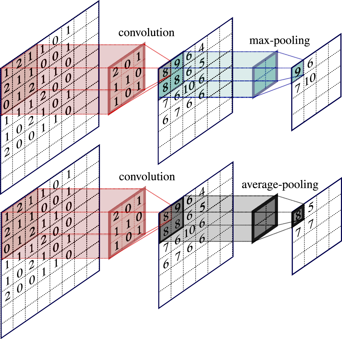
Figure 2. Operations carried out by the convolution and pooling layers. A max-pooling layer picks the maximum number from the layer input within a selected window, while an average-pooling layer computes average values over the selected window. In this example, the 8 × 8 input layer is reduced to a 6 × 6 output layer after going through a convolution layer consisting of a single 3 × 3 filter array of trainable parameters that takes stride 1. This output layer becomes the input layer with respect to either the max-pooling or average-pooling layer that each consists of a single 2 × 2 filter array of stride 2. The final output layer (rounded off for illustration purposes) is therefore a 4 × 4 numerical array.
Download figure:
Standard image High-resolution imageOverfitting can be an issue in machine learning, in which case the neural networks are prone to fitting training datasets much better than unseen ones. It is therefore essential to regulate network training by keeping the problem of overfitting in check so that the resulting trained models have high predictive power. This problem often arises when the neural network is deep. The addition of dropout layers has been proven to be an effective method for combating overfitting [82–84], which randomly exclude trainable parameters. More recently, it has been demonstrated that NN training can be further enhanced by adding BN layers. This was supported not only by the initial observation that the distribution of layer input values are stabilized with BN [85], but also by the even more relevant finding that the gradient landscape of the network loss function (the figure of merit quantifying the difference between the actual output value and that computed by the network) seen by the optimization routine that trains the network becomes smoother [86], making training much more stable.
All trainable parameters in the relevant neural layers of ICCNet and FidNet are optimized using a variant of stochastic gradient descent known as NAdam [87], where the network gradients are computed in batches of the training data. To prepare ICCNet training input datasets, for von Neumann measurements of a fixed number (K) of bases considered in sections 4.1 and 4.2, the initial network input X is an m × K(d2 + d) matrix that contains m training datasets, each recording the K measured bases and corresponding relative frequencies  (∑j
νjk
= 1). To encode the measurement bases, we regard all bases as some unitary rotation
(∑j
νjk
= 1). To encode the measurement bases, we regard all bases as some unitary rotation  of the standard computational basis
  , where U1 = 1. These unitary operators are then logarithmized in order to obtain their Hermitian exponents Hk
= −i log Uk
(H1 = 0), from which the diagonals and upper triangular real and imaginary matrix elements are extracted. Each row of X is thus a flattened K(d2 + d)-dimensional row of real numerical values formatted properly to encode U1, U2,..., UK
, ν01,..., νd−1 1, ν02,..., νd−1 2,..., ν0
K
, ..., νd−1 K
in this order. This input matrix is then processed into a
, where U1 = 1. These unitary operators are then logarithmized in order to obtain their Hermitian exponents Hk
= −i log Uk
(H1 = 0), from which the diagonals and upper triangular real and imaginary matrix elements are extracted. Each row of X is thus a flattened K(d2 + d)-dimensional row of real numerical values formatted properly to encode U1, U2,..., UK
, ν01,..., νd−1 1, ν02,..., νd−1 2,..., ν0
K
, ..., νd−1 K
in this order. This input matrix is then processed into a  square training array of elements, which is then fed to ICCNet (see figure 3). Zeros are padded to this array in order to complete the square. Similarly, for a fixed set of L projective measurements discussed in section 4.3, analogous arguments lead to the necessary
  input square training array. For each dimension, the randomly generated full-rank state Z needed to solve (2.1) is fixed during the training and testing stages.

Figure 3. A juxtaposition of (a) a 33 × 33 pixelated ICCNet input-data image, which encodes a four-qubit POVM containing K = 4 bases and corresponding probabilities, and (b) a down-sampled photograph of a stuffed toy of the same resolution. Here, the ICCNet input-data image is generated by proportionately scaling all numerical values in the square training array X to values between 0 and 255 only for the purpose of illustrative comparison.
Download figure:
Standard image High-resolution imageOn the other hand, training the FidNet requires input information about not only the measured bases (or projectors) and their corresponding data, but also the additional m target states to be included as inputs, one for each dataset. The correct dimensions of the training arrays are  or
or  respectively for basis and projective measurements. We note that to predict fidelities for simulated test datasets of d = 16, 32 and 64 as shown in figures 7 and 8,
For all purely-simulation figures, FidNet training is done with target states defined by the true states that generated the simulated training datasets. On the other hand, for all experimental results in figure 9 9, FidNet training is carried out simultaneously with the target states derived from the corresponding true states and those that deviate from them in order to account for systematic errors more effectively and improve average prediction accuracy. The list of hyperparameters that define the architectures of ICCNet and FidNet, as well as the technical analyses of network input-data generation and network training are given in sections II and III of supplementary material (https://stacks.iop.org/NJP/23/103021/mmedia).
Once an IC set of measurements are performed and assessed with ICCNet and FidNet, the density matrix representing the final state estimator may be obtained using the accelerated projected-gradient algorithm developed in [75]. Alternatively, it is possible to append our networks with additional conditional generative networks to yield the density matrix [62, 63].
3. Experiments
3.1. Spatial-mode photonic systems
Apart from evaluating simulation test datasets, we also run the trained ICCNet and FidNet models to benchmark real experimental datasets. In the first group of experiments, we showcase the accuracy of ICCNet and FidNet predictions on experimental data acquired from an attenuated laser source prepared in quantum states projected onto Hermite–Gaussian spatial-mode bases of various dimensions d. With this group of experiments, for the sake of variety, we shall consider measurement bases that are obtained from adaptive compressive tomography (ACT). These are eigenbases of the state that minimizes the von Neumann entropy subject to the same SDP constraints in (2.1). It has been demonstrated that successive measurements of such eigenbases result in a fast convergence of sCVX [52, 53]. An explicit protocol to construct these bases is given in section I of supplementary material.
The Hilbert space of photonic spatial degrees of freedom is typically discretized using an appropriate basis of transverse modes. To produce high-dimensional quantum states we attenuate an 808-nm diode laser, filter the resulting radiation with a single-mode optical fiber and then adjust the spatial structure of the light field with a spatial light modulator (SLM, see figure 4). The holographic approach [88] allows us to transform the incident light into arbitrary transverse modes by controlling the phase pattern on the SLM's display.

Figure 4. Experimental scheme to generate and characterize spatial photon states. Attenuated radiation of laser diode is spatially filtered by a single-mode optical fiber (SMF1) and directed on the first spatial light modulator (SLM1). Hologram displayed on the SLM1 transforms the fundamental fiber mode into the desired superposition of Hermite–Gaussian beams defining the particular quantum state of photons. The iris placed in the middle of the telescope with unit magnification (lenses L1 and L2) is used to clean the structured beam from the undiffracted light by selection of the first order of diffraction at the far-field plane of the SLM1. The second light modulator (SLM2) followed by a single-mode optical fiber (SMF2) and a single photon counter (D) plays a role of spatial detector, which realize a projective measurement by the right choice of a hologram on the second SLM display.
Download figure:
Standard image High-resolution imageWe work with Hermite–Gaussian (HG) modes HGnm (x, y), which are the solutions to the Helmholtz equation in Cartesian coordinates (x, y) and form a complete orthonormal basis. By bounding the sum of beam orders n + m, we restrict the dimension of the generated quantum systems. Since holograms displayed on the SLM make use of a blazed grating, in order to select the first diffraction order, we place an iris in the middle of the telescope, where different diffraction orders are well separated. Using a second SLM, a single-mode optical fiber, followed by a single photon counting module, we realize a well-known technique of projective measurements in the spatial-mode space [89]. These allows us to also conveniently implement general ACT basis measurements in arbitrary dimensions.
3.2. Multiphoton systems
In the second group of experiments, we switch to a different flavor of informational completeness by discussing two-mode photon-number states. In particular, we look at quantum states of up to three photons occupying two optical modes. Such three-photon states were of interest in the study of high-order quantum polarization properties beyond the Stokes vectors [90]. The resulting Hilbert space is effectively four-dimensional and spanned by the set  . Here nH and nV denote the number of photons in the horizontal and vertical polarization modes, respectively.
To perform tomography on the multiphoton quantum states, expectation values of a set of 16 rank-one projectors are measured. In principle, any set of 16 linearly independent projectors are suitable for a complete characterization of arbitrary four-dimensional states without ICC. For these experiments, we define each projector Πj
by a ket  , where
  and the other unobserved counterpart
  are photonic creation operators derived from an SU(2) unitary operator
  according to the transformation

and  and
and  are the creation operators of the horizontal and vertical polarization modes [91]. Clearly, ∑j
Πj
≠ 1 this time, as the projectors are independently measured.
are the creation operators of the horizontal and vertical polarization modes [91]. Clearly, ∑j
Πj
≠ 1 this time, as the projectors are independently measured.
Figure 5 depicts the experimental setup to generate and characterize three-photon states. Four photons are produced through double pair emission of non-collinear SPDC process. The initial state is prepared in |2, 2⟩ by combining two horizontally polarized photons and two vertically polarized photons with a PBSTo ensure that the photons are indistinguishable in the frequency domain, interference filters of 3 nm bandwidth centered at 780 nm are placed before sending the photons into the PBS. The four photons are then reduced into three photons by detecting a photon at D1 and the reflected three photons from a PPBS are in the state of  . The PPBS perfectly reflects vertically polarized photons and reflects 1/3 of horizontally polarized photons. The HWP setting of θ1 = 0° leaves the state unchanged, whereas the setting of θ1 = 45° transforms the state into
  . In addition, the mixed state
  is obtained by incoherently adding the relevant pure states through post-processing. These three-photon states are used to demonstrate the performances of ICCNet and FidNet in figure 9(b).

Figure 5. Experimental scheme to generate and characterize three-photon states. Two horizontally polarized photons and two vertically polarized photons, produced by the double-pair emission of non-collinear spontaneous parametric down-conversion (SPDC) process, are spatially combined with a polarizing beam splitter (PBS), thereby producing the four-photon state  . After detecting a single photon at detector D1, the reflected three-photon system from a partially-polarizing beam splitter (PPBS) are prepared in a particular quantum state, determined by the half-wave plate (HWP) angle θ1. For state characterization, four-fold coincidence counts at detectors D1, D2, D3, and D4 are acquired for all 16 rank-one projectors pictorialized in figure 6. These measurement projectors are determined by the HWP and quarter-wave plate (QWP) angles of θ2 and θ3 in the table with a PBS and beam splitters (BS).
Download figure:
Standard image High-resolution imageExperimentally [90], the three-photon states were characterized by acquiring the four-fold coincidence counts at D1, D2, D3, and D4 for 16 rank-one projectors after passing through a PBS and BS. The SU(2) unitary operators  that define the projectors
  according to rule (3.1) are determined by the QWP and HWP angles of θ2 and θ3 inasmuch as
  , where the matrix representations for the wave plates are given by

In our experiments, we consider SU(2) rotations that fairly distribute the single-photon component  on three Bloch-spherical circles parallel to the equatorial plane [90, 92] as shown in figure 6. The measurement angles that realize these projectors are given in figure 5.

Figure 6. Reduced visualization of the 16 two-photon measurement projectors on the single-qubit Bloch sphere. The projectors of three-photon states are defined as  in accordance with equation (3.1). The projection states are chosen to equally distribute the corresponding single-photon component pure states
  on the equatorial great circle and two small circles on the Bloch sphere, together with the south pole.
Download figure:
Standard image High-resolution image4. Results
4.1. Simulations—neural-network performances
We first present performance graphs of ICCNet and FidNet in figure 7 based on two sets of simulations on four-qubit states (d = 16) using random measurement bases generated with the Haar measure for the unitary group (see section I of supplementary material), and bases found using ACT. In each set of simulations, for both cases where statistical noise is either absent or present, we collect simulation data of various number (K) of bases (sCVX is normalized to 1 at K = 1 by default), each case recording measurements of 5000 randomly-generated quantum states of uniformly distributed rank 1 ⩽ r ⩽ 3. The explicit CNN architecture employed is specified in section 2.2. The accurate fit between the actual computed values and those predicted by ICCNet and FidNet suggests that faithful neural network predictions of both the degree of informational completeness and fidelity are a definite possibility in both noiseless and statistically noisy environments. Sample codes for network training and evaluation with four-qubit simulation datasets are available online [93].

Figure 7. Performance of ICCNet and FidNet in the prediction of sCVX and  for different number (K) of measurement bases generated by (a) random unitaries sampled from the Haar unitary group and (b) adaptive unitaries from ACT, accompanied by 1-σ error bars derived from 50 simulated test experiments for each rank r that are not seen by the neural networks. The main plots correspond to perfect measurement data, whereas the insets show results under statistical noise with N = 1000 sampling copies per basis. Both the actual computed values and NN predictions are evidently in extremely good agreement.
Download figure:
Standard image High-resolution imageIn separate simulations on four- (d = 16), five- (d = 32) and six-qubit (d = 64) systems with random Haar measurement bases, numerical evidence presented in figure 8 shows that the computation times in sCVX NN predictions can be significantly reduced by about four orders of magnitude relative to ordinary SDP calculations, and this difference grows wider with larger dimensions. The corresponding ICCNet and FidNet performance graphs similar to figure 7 are given in section V of supplementary material.

Figure 8. Comparison of the average ICC computation time by carrying out the grayed subroutine (physical-probabilities extraction and SDP-based ICC) in figure 1 (unfilled markers) and a trained ICCNet model (solid markers) over many simulated experimental runs and states of various ranks. For d = 32 and 64, a set of 1000 datasets (N = 1000) each is used to acquire average computation times that are sufficiently representative (the sCVX and  graphs are separately presented in the supplementary material). These timing are obtained through CUDA 10.2 interfaced with the GPU-enabled TensorFlow 1.9 package on Python 3.5.3, with the Keras 2.1.6 frontend running on a twelve-core Intel(R) Xeon(R) CPU E5-2620 v3 at 2.40 GHz and an Nvidia GTX 1080 TI GPU of native settings. A trained FidNet model, on average, performs fidelity benchmarking in times that are roughly the same orders of magnitude. That the d = 16 neural-network time curve is between those for d = 32 and 64 is due to neural-network-architectural differences for different d values. Performance gaps are barely noticeable in practice.
Download figure:
Standard image High-resolution image4.2. Experimental performance with spatial-mode photonic states
For each value of d, we experimentally generated random pure states and construct their respective ACT measurement bases in order to evaluate the performance of ICCNet and FidNet, which were previously trained with 10 000 simulation datasets of random quantum states of uniformly distributed rank 1 ⩽ r ⩽ 3 and different K values. These simulated training datasets are modeled with statistical noise arising from a multinomial distribution defined by N = 5000 sampling copies per basis, which is close to the experimental average.
Owing to experimental noise, the resulting spatial-mode quantum states are, as a matter of fact, nearly pure but sufficiently low-rank. Figure 9(a) confirms that ICC and fidelity benchmarking with simulation-trained neural network models are accurate even with real experimental test data. One can observe the relative network-prediction stability of sCVX in contrast with that of  . This coincides with the expectation that while the fidelity is strongly affected by statistical noise and other imperfections such as systematic errors, the degree of informational completeness is more intimately related to the quantum measurements and rank of the quantum state, such that noise only introduces perturbations on the functional behavior of sCVX. Regardless, figure 9(a) shows that all predictions made by the simulation-trained ICCNet and FidNet models remain roughly within the error margins of actual computed values.

Figure 9. (a) The NN predictions of sCVX and  for spatial-mode photonic states of dimensions d = 4, 6 and 9. All graphs and 1-σ error bars of each dimension d are obtained from 15 experimental test states used to evaluate the networks. The average fidelity mapped out by FidNet lies closely with the actual computed curve. (b) Performances on three-photon systems are given for states
  ,
,  , and the rank-two
  in this order. All graphs and 1-σ error bars are obtained from 20 experimental test runs per quantum state. Despite the large error bars of the actual values owing to noise and experimental imperfections, the average fidelity curve is correctly identified by FidNet.
Download figure:
Standard image High-resolution image4.3. Experimental performance with multiphoton states
For every fixed number (L) of projectors chosen from the complete set of 16 defined in section 3.2, simulation datasets of 10 000 random d = 4 quantum states of uniformly distributed r are fed into both ICCNet and FidNet for training. These datasets are obtained from randomized sequences of the 16 projectors described above. Statistical noise is introduced into the simulation with multinomial distributions defined by N = 500 per projective measurement. To test the trained models and acquire prediction results depicted in figure 9(b), we make use of three different sets of 20 experimental runs outside the training datasets, each set corresponding to a different quantum state.
4.4. Noise training and reduction
Experimental noise due to imperfections and systematic errors are always present in any real dataset. Fluctuating deviations of NN predicted values from actual ones as observed in figure 9 arise from the lack of such experimental noise in all simulated training datasets, apart from purely statistical fluctuations, used to train ICCNet and FidNet.
When more knowledge about the noisy environment is acquired, data simulation from such knowledge may be carried out to improve the network predictions under such an environment. Here, we show that when some samples of experimental data that are sufficiently representative of the overall noise behavior can be spared for training, it is possible to train ICCNet and FidNet with both statistically-noisy simulated datasets and bootstrapped experimental datasets in order to learn the experimental noise effects approximately well and improve network predictions.
Bootstrapping entails using a given experimental dataset to generate numerous mock datasets using Monte Carlo procedures. More specifically, in the multinomial setting, the column
ν
k
of relative frequencies for the kth basis possess a Gaussian distribution of mean
p
k
and covariance matrix ![${\mathbf{\Sigma }}_{p}^{(k)}=[\mathrm{diag}({\boldsymbol{p}}_{k})-{\boldsymbol{p}}_{k}\enspace {{\boldsymbol{p}}_{k}}^{\mathrm{T}}]/N$](https://content.cld.iop.org/journals/1367-2630/23/10/103021/revision3/njpac1fcbieqn46.gif) for sufficiently large N owing to the central limit theorem, where diag(⋅) forms a diagonal matrix whose diagonals are defined by the argument. A direct substitution of
ν
k
for
p
k
leads to the following simple rule for bootstrapping experimental ACT datasets from Hermite–Gaussian mode photonic system:
for sufficiently large N owing to the central limit theorem, where diag(⋅) forms a diagonal matrix whose diagonals are defined by the argument. A direct substitution of
ν
k
for
p
k
leads to the following simple rule for bootstrapping experimental ACT datasets from Hermite–Gaussian mode photonic system:  , where
w
k
is a column of random variables collectively distributed according to the Gaussian distribution of zero mean and covariance matrix
, where
w
k
is a column of random variables collectively distributed according to the Gaussian distribution of zero mean and covariance matrix  where
where  is to be evaluated with the measurement relative frequencies of the particular kth basis and N is set to 5000, which is the estimated number of copies per ACT basis considered in section 4.2. The operation
  is a composition of absolute value of the argument followed by its sum normalization over 0 ⩽ j ⩽ d − 1 for the kth ACT basis. Finally, the states that produce the bases relative frequencies used in the bootstrapping procedure are different from the test states used to evaluate the network predictions.
Owing to a limited set of three-photon states, we adopt a different method to bootstrap experimental datasets acquired from these states. Since these datasets are obtained from measuring independent projectors, we randomly permute these projectors and their corresponding relative (unnormalized) frequencies in order generate new measurement sequences as mock datasets. The 16 projectors offer us a total of 16! permutations for each state, allowing us to conveniently generate an abundance of bootstrapped training datasets that are clearly different from those used for testing. By a similar token to the spatial-mode photonic systems, each relative frequency νl
here is a binomial random variable normalized by the number of copies N used to measure the lth projector. Therefore, bootstrapping these relative frequencies may be carried out by additive Gaussian random variables inasmuch as  , where wl
is a standard Gaussian random variable of zero mean and unit variance, and N = 500 is fixed as the estimated number of copies used to obtain the measured relative frequency for each projector, consistent with figure 9(b).
, where wl
is a standard Gaussian random variable of zero mean and unit variance, and N = 500 is fixed as the estimated number of copies used to obtain the measured relative frequency for each projector, consistent with figure 9(b).
Figure 10 shows the enhanced prediction performances of ICCNet and FidNet. To generate this figure, a total of 5000 simulated and 5000 bootstrapped datasets are employed (m = 10 000) for each group of experiments to train the networks for every value of K and L. These new plots indicate that slightly fluctuating NN prediction curves on noisy experimental data can be smoothened when bootstrapped information about the noisy environment is incorporated into the training.

Figure 10. The bootstrapped performance of ICCNet and FidNet in predicting sCVX and  for the same test datasets that are used in figure 9, where fluctuating features are generally smoothened with bootstrapped noise training.
Download figure:
Standard image High-resolution image4.5. Suppression of systematic errors
To end this section, we shall now discuss the implications of all presented results, especially the computation performance graphs shown in figure 8, as far as real-time experimental systematic errors are concerned [94, 95]. As analytical results are unavailable, we resort to numerical analyses on the effects of ICC-computation-time reduction on such errors. For this purpose, we provide an important example of a kind of systematic drift phenomenon that is highly typical in optical fibers that carry spatial-mode photons, such as those of Hermite–Gaussian modes discussed in this article.
Focusing only on the transverse plane relative to the propagation direction of a laser beam, a given Hermite–Gaussian mode function um (x) of order m in the spatial x-coordinate is given by [96]

with w0 being the beam waist, and  a degree-m Hermite polynomial in x. Upon using the ket notation, one can express the mode function in the familiar manner inasmuch as ⟨x|m; 0⟩HG = um
(x). An ideal fiber would carry spatial-mode photons of a mode function that has a stable center point, which is usually set at the Cartesian origin as in (4.1). In real experiments, however, a main source of time-dependent systematic errors is transversal displacements of um
(x) away from the origin [97, 98], which we may approximately model as random Wiener processes. Such displacements would distort the originally intended true state. Suppose that a basis ket
a degree-m Hermite polynomial in x. Upon using the ket notation, one can express the mode function in the familiar manner inasmuch as ⟨x|m; 0⟩HG = um
(x). An ideal fiber would carry spatial-mode photons of a mode function that has a stable center point, which is usually set at the Cartesian origin as in (4.1). In real experiments, however, a main source of time-dependent systematic errors is transversal displacements of um
(x) away from the origin [97, 98], which we may approximately model as random Wiener processes. Such displacements would distort the originally intended true state. Suppose that a basis ket  is displaced away from the origin by a, it is shown in section IV of supplementary material that the resulting displaced
  , where
  , possesses the following transformation function

where n> = max{m, l}, n< = min{m, l}, and

is Kummer's confluent hypergeometric function. This result reduces to that in [97] for the m = 0 special case. The complete two-dimensional transverse profile of a Hermite–Gaussian mode in space is therefore described by the mode function um,n
(x, y) ≡ um
(x)un
(y), where the corresponding displaced kets  exhibit the transformation

where the coefficients are pair-products of one-dimensional transformation functions as in (4.2). Components of the two-dimensional displacement  are assumed to be independent. After a period of time t, the noisy true state
  is now defined in the displaced Hermite–Gaussian basis of some displacement
a
(t). The same type of disturbances apply to the POVM outcomes since they are implemented digitally using SLMs with the same beams.
is now defined in the displaced Hermite–Gaussian basis of some displacement
a
(t). The same type of disturbances apply to the POVM outcomes since they are implemented digitally using SLMs with the same beams.
In the experiments that gathered data used in plotting figure 9(a), the root-mean-square displacement of the Hermite–Gaussian beam center was measured to be about 5% of the beam waist w0 after a period of 24 hours. This approximately coincides with a model of a Wiener process specified by the random displacement variable
a
(t) =
a
(t − 1) +
b
(t − 1), which is a cumulative temporal sum of random variables
b
(t) that are each distributed according to the standard Gaussian distribution defined by the standard deviation σ ≈ w0/95 when the time coordinate t is in units of an hour. Figure 11 shows the Hermite–Gaussian beam-profile center displacement and fidelity curves in time t for various dimensions d, where  is the product of the individual dimensions d0 of the truncated Hilbert space spanned by the finite set of Hermite–Gaussian basis kets of orders 0 ⩽ m, n ⩽ d0 − 1. In actual experiments, there most likely exist other time-dependent sources of errors not modeled here that could worsen the fidelities.

Figure 11. (a) Random single-direction displacements of the beam-profile center shows an increasing variance around the zero-displacement origin that is expected of random-walk Wiener processes. Such variance drifts give rise to the fidelity curves with respect to ideal true states ρ in (b) for the noisy true states  and those in (c) for the reconstructed estimators
  , in contrast to the driftless scenarios in (d).
Download figure:
Standard image High-resolution imageTo appreciate the significance of systematic-error suppression, we consider a quantum processor that utilizes Hermite–Gaussian beams as a source for producing high-dimensional initial states for quantum computation. Suppose that the processor is running continuously under server conditions, and maintenance is carried out before significant systematic drifts are anticipated. Whenever the processor refreshes after each set of computations is completed, the newly prepared initial state ρ undergoes compressive state tomography to ensure that it is within the expected error margins.
As an instructive example, we consider at an eight-qubit processor controlled by a d = 256 Hermite–Gaussian source [99]. Each projector exposure time is about 1.5 s so that the measurement time of K von Neumann bases is tmeas = 1.5Kd = 1920 s. Preliminary calibration indicates that such an exposure period yields N = 1000d = 2.56 × 10⁵ state copies per basis. For a realistic error modeling, the expressions of tmeas and N in d were calibrated from the actual setup used to collect our experimental data for figures 9 and 10. We focus on the preparation of pure states, each of which requires only K = 5 random bases for an IC reconstruction [53], the average time, estimated over five random sets of K = 5 bases, for an ICC verification (two SDPs) is tSDP = 4000 s using the personal computer with hardware specification given in the caption of figure 8. After carrying out the basis measurements and ICC, the final state estimator  is given by the ML estimator that takes an average of tML ≈ 240 s to generate using the accelerated projected-gradient algorithm in [75], which is insignificant in comparison to tSDP. The time for each round of quantum computation depends on the actual application. For simplicity, we assume that each round of quantum computation is executed almost instantly since no classical post-processing is needed. From these specifications, we note that tSDP ≈ 2tmeas, and the prefactor grows with d > 256. Therefore, in the case of d = 256, replacing the two SDP algorithms in ICC with a trained ICCNet would shave about 66% of the total computation time off. For larger dimensions, if so desired, the ML estimation procedure may be completely replaced with trained conditional generative networks [62, 63] to eliminate tML.
Figure 12 shows the fidelity of the estimator  with the generated initial state ρ before every quantum-computation step (Nc of them in total). The graphs highlight the adverse effects of systematic errors when initial-state verification takes too long. Hence, compressive tomography performed with trained neural networks provides a better solution to real-time device certification with a higher fidelity stability, so that quantum computation can run much more smoothly with a greater Nc output before drift maintenance is applied.

Figure 12. The fidelity  of the input state ρ with (a) the noisy true state
  , and that with (b) its IC estimator
  , before each round of quantum computation commences (step labeled by Nc) for an eight-qubit (d = 256) processor executed with Hermite–Gaussian optical sources. Using ICCNet in place of SDP-based ICC not only triples the computation output Nc in a given period of time (assuming negligible quantum-computation timescales), but also maintains a much more stable fidelity for the same number of computations. All 1-σ error regions are computed from 10 different runs.
Download figure:
Standard image High-resolution image
5. Concluding remarks
We took advantage of the universality of convolutional networks to train two neural networks that can very efficiently certify a low-measurement-cost quantum-state characterization scheme. These networks can respectively benchmark the quantum completeness of a given set of measurement outcomes and corresponding data for reconstructing an unknown quantum state, as well as the resulting fidelity without explicitly carrying out the state reconstruction. Our machine-learning-assisted scheme therefore allows experimentalists to rapidly assess the sufficiency of measurement resources for an unambiguous characterization of arbitrary quantum states and achieve accelerated real-time verification without having to perform any optimization routine during the experiment. This becomes essential for many practical quantum tasks that do require fast execution times to avoid noise accumulation and drifts.
An arguably interesting problem would be to minimize the time required to acquire the trained neural networks. This includes both the training time and the generation of adequate training datasets. While the former can now be easily parallelized with graphics processing units, the latter involves two rounds of semidefinite programming per dataset as discussed in section 2.1, the acceleration of which is still a subject of ongoing research [100].
On the other hand, while classical algorithms for these procedures have worst-case polynomial time complexities in the dimension of the Hilbert space, it is known [101] that quantum algorithms can execute SDPs with polylogarithmic time complexities in the dimension. This immediately reveals the possibility of completely transforming the neural networks employed here, or part thereof, into their quantum counterparts (fused with the training-data processing procedures that use quantum semidefinite programming) that could assimilate into a much larger set of networks for a grander purpose. Practical feasibility in implementing such extended quantum neural networks still remains to be seen.
Note.—Nearing the submission of our work, we discovered another very recent preprint reference [102] that purely discusses the estimation of the fidelity with FC networks. Apart from the clear distinction in architectures, we remark that while the networks in this reference were specifically trained for Pauli measurements, our CNN-based FidNet is compatible with generalized measurement inputs that can be readily used in parallel with ICCNet or any other quantum task that relies on arbitrary measurements. The objectives of both works are hence very different. The next key distinction is network training, which in this reference is based on categorical training that splits the continuous fidelity range into small intervals. As mentioned in the preprint itself, network training can be slow when the intervals are too small. In our current work, FidNet directly computes the fidelity values without such output splitting, and hence training efficiency is not sacrificed for prediction accuracy.
Acknowledgments
YST, SS and HJ acknowledge support by the National Research Foundation of Korea (Grant Nos. 2019R1A6A1A10073437, 2019M3E4A1080074, 2020R1A2C1008609, and 2020K2A9A1A06102946) via the Institute of Applied Physics at Seoul National University, and by the Institute of Information & Communications Technology Planning & Evaluation (IITP) grant funded by the Korea government (MSIT) (Grant Nos. 2020-0-01606 and 2021-0-01059). GL acknowledges support by the Center of Excellence ⟪Center of Photonics⟫ funded by the Ministry of Science and Higher Education of the Russian Federation, Contract No. 075-15-2020-906. YK and Y-HK acknowledge support by the National Research Foundation of Korea (Grant No. 2019R1A2C3004812) and the ITRC support program (IITP-2020-0-01606). LLSS acknowledges support from European Union's Horizon 2020 research and innovation program (ApresSF and STORMYTUNE) and the Ministerio de Ciencia e Innovación (PGC2018-099183-B-I00). The MSU team acknowledges support from the Russian Foundation for Basic Research (RFBR Project No. 19-32-80043 and RFBR Project No. 19-52-80034) and support under the Russian National Technological Initiative via MSU Quantum Technology Centre. SSS and SPK acknowledge support by the Development Program of the Interdisciplinary Scientific and Educational School of Lomonosov Moscow State University 'Photonic and quantum technologies: Digital medicine'.
Data availability statement
The data that support the findings of this study are available upon reasonable request from the authors.