


Abstract
The forthcoming generation of multi-petawatt lasers opens the way to abundant pair production by the nonlinear Breit–Wheeler process, i.e. the decay of a photon into an electron–positron pair inside an intense laser field. In this paper we explore the optimal conditions for Breit–Wheeler pair production in the head-on collision of a laser pulse with gamma photons. The role of the laser peak intensity versus the focal spot size and shape is examined keeping a constant laser energy to match experimental constraints. A simple model for the soft-shower case, where most pairs originate from the decay of the initial gamma photons, is derived. This approach provides us with a semi-analytical model for more complex situations involving either Gaussian or Laguerre–Gauss (LG) laser beams. We then explore the influence of the order of the LG beams on pair creation. Finally we obtain the result that, above a given threshold, a larger spot size (or a higher order in the case of LG laser beams) is more favorable than a higher peak intensity. Our results match very well with three-dimensional particle-in-cell simulations and can be used to guide upcoming experimental campaigns.
Export citation and abstract BibTeX RIS

Original content from this work may be used under the terms of the Creative Commons Attribution 4.0 licence. Any further distribution of this work must maintain attribution to the author(s) and the title of the work, journal citation and DOI.
1. Introduction
Abundant electron–positron pair production is among the most exotic and striking processes of extremely high-intensity laser interaction with light and/or matter that will be made possible by the emerging class of multi-petawatt (multi-PW) laser systems [1]. Under conditions envisioned for forthcoming facilities such as Apollon [2], CoReLS [3], ELI [4], OMEGA-EP OPAL [5], XCELS [6] and zeus [7], the dominant process leading to pair production is nonlinear Breit–Wheeler, i.e. the decay of a high-energy photon, as it interacts with the strong laser field, in an electron–positron pair [8, 9].
In the last decade, various simulation campaigns have been conducted to help design the future experiments to efficiently drive this process, an effort that was largely made possible and supported by particle-in-cell (PIC) simulations accounting for quantum electrodynamics (QED) processes [10–15]. Several configurations have been considered. Electron-seeded electromagnetic/QED cascades in the collision of two counter-propagating laser pulses, a setup originally proposed by Bell and Kirk [16], have attracted particular attention [11, 14, 17–20] as such cascades were identified as a possible limitation on the attainable intensity of high power lasers [21]. This setup was further built upon considering either the use of plasma channels [22] or the collision of multiple laser pulses [23–25]. All these works considered multiple laser beams, but electromagnetic cascades were also predicted considering the direct irradiation of a solid target by a single, extremely intense laser pulse, a situation that leads to the production of dense pair plasmas [26] (see also [27] for an application to laboratory astrophysics). In these cases, the solid target, an overdense plasma acts as a mirror and pair production is efficiently achieved in the field of the incident and reflected laser light at the target front [28].
All the previously discussed configurations considered cascades seeded by electrons initially at rest in the laboratory frame. The seed electrons, strongly accelerated in the electromagnetic fields of laser pulses with extreme intensity (typically ∼1024 W cm−2), gain energies at the GeV-level (as expected, at such intensities, from the ponderomotive scaling) and are the source (via nonlinear Compton scattering) of the high-energy photons triggering pair production. Another possible path toward pair production in the laboratory relies on an already existing high-energy electron or photon source. The two latter schemes are related, as photons with energy of the order of the electron one are produced via nonlinear Compton scattering of electrons in the intense laser fields [29–33]. Indeed, this configuration was exploited in the seminal E-144 experiment at SLAC [34], where the head-on collision of 46.6 GeV electron beams with TW laser pulses gave the first direct demonstration of nonlinear Breit–Wheeler pair production. However, the laser intensity in this experiment was only marginally relativistic, and very few positrons were produced (∼100 positrons over nearly 22 000 electron-laser collisions).
Combining GeV-electron beams with PW and multi-PW lasers will allow to extend this study deep into the relativistic regime, as investigated in [35] that numerically demonstrated the possibility of producing extremely bright high-energy photon sources as well as positrons bunches for laser intensities ≳1022 W cm−2, in conditions relevant to the Apollon facility. This configuration was further studied theoretically and via PIC simulations in [36–38], while the possibility to produce pairs via nonlinear Breit–Wheeler with high-energy photons from a Bremsstrahlung source was presented in [39].
In this paper, we focus on the study of nonlinear Breit–Wheeler pair production following from the head-on collision of an extremely intense laser (intensities in the range 1021–1025 W cm−2) with a burst of gamma photons (with energies ranging from 100 MeV to few 10 s of GeV). In contrast to [39], where the authors focused on the optimization of the photon source, we consider here the high-energy photon burst as given (only its energy will vary), and do not discuss its origin (various sources of high-energy photons have been proposed [25, 39–46]). Rather, we aim to optimize the conditions of interaction with the colliding high-intensity laser. Motivated by experimental constraints, we investigate the optimal conditions for pair production varying the laser polarization, focusing, spatial or temporal profiles, always considering a fixed laser energy.
In particular, special attention will be paid to the use of Laguerre–Gauss (LG) beams, which have recently attracted the interest of the ultra-high intensity laser-plasma community [38, 47–50] for their ability to carry orbital angular momentum (OAM) [51]. These beams, that emerge as eigen-modes of the paraxial equation, have unique properties, such as a ring-shaped intensity distribution and the large OAM, that could have an impact on pair production. It was for instance demonstrated in [38] that the collision of an electron beam with a LG beam can lead to efficient production of gamma rays carrying large OAM, to enhanced secondary radiation emission and pair production. However, that study was performed at constant maximum intensity, so it is hard to distinguish the impact of the increased energy (up to 3× higher for the LG beam) from the role of the laser spatial profile itself. We will discuss this aspect in detail in this paper.
Because of the remarkable number of free parameters to study (polarization, focusing, spatial and temporal profile) and the complex spatio-temporal dependence of the electromagnetic fields of LG beams, it is useful to develop and validate a reduced analytical model for pair creation (see reference [52] for an analytical study of the Breit–Wheeler pair production process in a Gaussian beam). Starting from the probability for a given high-energy photon to decay in an electron–positron pair while it crosses an extremely intense laser pulse, we propose a simple, yet accurate, model to compute the number of pairs created during this interaction. The computation relies on three assumptions. (i) The electron–positron pair production rates are obtained in the locally constant cross-field approximation [53]. (ii) The newly created charged particles do not further contribute to pair production. (iii) The potentially complex electromagnetic fields explored by the high-energy photons as they cross the laser pulse are approximated, assuming that each photon sees a succession of single half-periods of monochromatic plane waves, the field amplitude of each half-period being computed so that both the temporal and spatial profiles of the laser pulse at focus are accounted for. As will be further discussed in this work, these assumptions are well satisfied for a wide range of parameters of interest for this study and currently accessible laser parameters. Our model goes further than previous studies [36, 53] as it accounts for arbitrary polarization and spatio-temporal profile of the laser beam, and it is not limited to small pair production probability and/or rate.
Three-dimensional PIC simulations performed with the code SMILEI [54] and embarking the relevant QED modules [15] are presented and validate our model. Assumptions (ii) and (iii) are shown to hold under conditions relevant to ultra-short laser pulses (up to few tens laser cycles) typical of the Ti:sapphire technology. Assumption (ii) holding is of particular importance as it demonstrates that, under conditions relevant to forthcoming ultra-short laser facilities, the high-energy-photon-laser interaction proceeds essentially in a regime which we refer to as the soft-shower regime [55]. Furthermore, our PIC simulations allow to test our model against complex laser pulse geometries, e.g. considering LG beams, showing that assumption (iii)—which is at the core of the simplification of our model—provides accurate predictions even for non trivial electromagnetic field configurations.
The proposed model and performed study make it possible to clearly identify the laser parameters and high-energy photon energy that optimize pair production for a given laser energy. This work also highlights the conditions in which either stronger focusing or increased gamma photon energy does not improve the production of primary pairs.
The paper is structured as follows. In section 2, we introduce the key properties of the nonlinear Breit–Wheeler process, and we propose a reduced model for pair creation in the head-on collision between gamma photons and a plane wave with arbitrary polarization. The possibility to account for a time envelope of the laser field is also considered and the model is benchmarked against 1D PIC simulations. In section 3 we consider the effect of the spatial dependence of the laser field. Both LG and Gaussian beams are considered and we introduce the notion of a total cross-section for which we propose a reduced model, shown to be in very good agreement with 3D PIC simulations. The optimal conditions for pair creation with respect to the laser geometry and intensity are also discussed. In section 4 we then use our model to discuss pair production on upcoming Ti:sapphire laser facilities, before giving our conclusions in section 5.
2. Reduced model for pair production in a time-varying background field
This section provides the theoretical framework for describing nonlinear Breit–Wheeler pair production, and aims to establish a simple model for pair production in a time-varying background field. Throughout this section, we consider the head-on collision of high-energy gamma photons with a strong, optical, laser pulse (also referred to as the background field). In addition to exact expressions, we provide practical formulae relevant to forthcoming high-power laser facilities, focusing on optical laser systems with micrometric wavelength λ, with relativistic field strength a0 = eE0/(me
cω) ≫ 1 (with ω = 2πc/λ the background field angular frequency), corresponding to I0
λ2 well beyond 1018 W cm−2 μm−2, with  the laser intensity. Note that SI units are used throughout this work: e, me and c denote the elementary charge, electron mass and speed of light in vacuum, respectively,
  0 the vacuum permittivity, re = e2/(4π0
me
c2) the classical radius of the electron, τe = re/c the time for light to cross re, ℏ the reduced Planck constant and α = e2/(4π0
ℏc) the fine-structure constant.
0 the vacuum permittivity, re = e2/(4π0
me
c2) the classical radius of the electron, τe = re/c the time for light to cross re, ℏ the reduced Planck constant and α = e2/(4π0
ℏc) the fine-structure constant.
2.1. Pair production instantaneous rate and probability
Nonlinear Breit–Wheeler is the dominant QED process leading to electron–positron pair production from the collision of a high-energy photon with a strong (optical) laser pulse [56, 57]. As discussed in reference [53], for a relativistically intense background field, a0 ≫ 1, the local constant field approximation holds and the pair production probability can be computed by integrating the instantaneous pair production rate. For a high-energy photon propagating with velocity c, normalized energy γγ = ℏωγ /(me c2) and instantaneous quantum parameter

where  is the Schwinger field and E and B denote the electric and magnetic fields at the photon position. The instantaneous pair production rate is given by (see, e.g. references [58, 59]):

where W0 = 2α2/(3τe). For a fixed value of the quantum parameter χγ , the rate is inversely proportional to the gamma photon energy γγ , and depends non-trivially on χγ through the function

with μ = 2/[3χγ ξ(1 − ξ)] and Kn (x) the modified Bessel function of the second kind. This function, shown in figure 1(a), can be well approximated (within less than 1% from the numerically computed values for χγ ∈ [10−2, 103]) by 5

The denominator in equation (4) provides a simple improvement of the well known Erber approximation [60], which also allows to recover the correct asymptotic behavior (dashed grey lines in figure 1(a)) of b0(χ):


with  and c2 = 32/345Γ4(2/3)/(56π2) ≃ 0.569 (Γ(x) denoting the gamma function).

Figure 1. (a) Dependence of b0(χγ
) on the photon quantum parameter χγ
as defined by equation (3) (black line) and asymptotic behaviors given by equations (5) and (6) (grey dashed lines). (b) Dependence of  (equation (19)) on the maximum photon quantum parameter χ0 (as defined by equation (13)), for a linearly polarized (LP) background field (ɛ = 0, black line) and a circularly polarized (CP) background field (ɛ = ±1, blue line). Dashed lines show the asymptotic behavior given by equations (22) and (23) for the LP case. The inset highlights the values of χ0 for which LP (χ0 < 2.52) or CP (χ0 > 2.52) gives higher pair production probability and the relative difference of
  (in absolute value) between the two cases.
Download figure:
Standard image High-resolution imageThe quantity WBW defined by equation (2) is the instantaneous rate of pair production, so that considering, at a time t0, a given number N0 of identical high-energy photons entering a strong background field, the number of photons Nγ remaining at later times t > t0 satisfies the rate equation:

where both Nγ and WBW depend on time (the latter when the high-energy photons explore electromagnetic fields with spatial and/or temporal variations). Note that equation (7) does not account for subsequent radiation from the produced pairs, which will be verified to be accurate for the investigated parameter range in section 3. The solution to this equation reads

from which one can derive the probability P(t0, Δt) = 1 − Nγ (t0 + Δt)/N0 for a given high-energy photon to decay into an electron–positron pair between time t0 and t0 + Δt:

When the time-integrated rate (i.e. the integral term in equation (8)) is small, it can be assimilated to the probability P(t0, Δt), as  . This leads some authors to refer to WBW as the pair production probability per unit time. While this is correct in the limit P(t0, Δt) ≪ 1, it leads to inconsistencies as the probability increases and the time-integrated rate assumes values greater than unity (see, also, references [53, 61–63]). Hence, throughout this work, we will distinguish pair production rate (as defined by equation (2)) and probability (as defined by equation (9)).
2.2. Pair production probability in an arbitrarily polarized plane wave
Let us now focus on the case of a high-energy photon colliding head-on with an ultra-intense laser pulse described by a plane wave (propagating in the  -direction), with electric field:

magnetic field  , and polarization ellipticity ɛ ∈ [−1, 1]. It takes the particular values ɛ = ±1 for a CP wave (± standing for opposite helicities), and ɛ = 0 for a LP wave (
 denoting by convention the direction of polarization). It is important to stress that our choice of parametrisation (equation (10)) ensures that the laser energy is the same for any value of ɛ. On the contrary,
  measures the maximum laser electric field amplitude and varies with the ellipticity.
When a high-energy photon collides with such a laser field (we define t0 = 0 as the time at which the photon enters the background field), the value of its quantum parameter

evolves in time as the photon explores regions with different electric and magnetic field amplitude (here zγ
(t) denotes the photon time-dependent position). In the case of head-on collisions ( ), the time-dependent photon quantum parameter reduces to

and

Note that, with our convention on the background field parametrization (equation (10)), χ0 denotes the maximum quantum parameter for the LP case only. For arbitrary ɛ, the maximum achievable quantum parameter χm is a decreasing function of |ɛ|

Note also that equation (12) takes a simple form when considering either a CP or a LP background field:


2.2.1. Decay probability after propagating through half a period of the background field
For arbitrary values of ɛ, χγ (t) is either a constant (for ɛ = ±1) or a periodic function of time with period τ/4 (we recall τ = 2π/ω) corresponding to the time for the high-energy photon to cross half a wavelength of the background field. It is thus convenient to compute the probability Pm of the high-energy photon to decay into a pair during this interval of time. Let us then consider a time tm at which the high-energy photon sees a maximum of the background electric field, and compute the probability Pm for the high-energy photon to decay into an electron–positron pair in between the times t0 = tm − τ/8 and t0 + τ/4 = tm + τ/8:

where Rm τ/4 is the time-integrate rate, while Rm denotes the average rate.
Let us stress that the dimensionless quantity W0/(2ωγγ ) in equation (17) is of order 1 for optical background fields (with micrometric wavelength λ) and GeV-level high-energy photons:

The probability Pm , that measures the contribution of a single field maximum, depends on the integral quantity

which, for a given polarization ellipticity ɛ, is a function of χ0 only as shown in figure 1(b) for LP (black line) and CP (blue line).
This integral is the key object to compute the pair creation probability and can be calculated either numerically or by means of an approximated formula as described in the following. In appendix  can be written in the approximate form:
where χm
is defined in equation (14) and  is the error function. The function F(s) emerges from the saddle point approximation used to compute the integral when the main contribution comes from the vicinity of the field maximum. It varies slowly with s, as
  for s ≪ 1 and F(s) → 1 for s → +∞. In equation (20), F(s) takes for argument sɛ
(χm
), with
for s ≪ 1 and F(s) → 1 for s → +∞. In equation (20), F(s) takes for argument sɛ
(χm
), with

where b0'(χ) denotes the derivative of b0(χ) and c(χ) is a slowly varying function of χ, as  for χ ≪ 1 and c(χ) → 1 for χ → +∞.
Equation (20) is exact for CP background fields (ɛ = ±1) for which s±1(χm
) → +∞, so that  . Moreover it allows to recover the asymptotic behavior of equation (19) in the limiting cases of small and large quantum parameter χ0:

where we used equations (5) and (6), and  ,
,  and c5 = 32/345Γ4(2/3)/(56π) ≃ 1.789.
2.2.2. Total decay probability
As will be further discussed in section 2.3, considering parameters typical of the upcoming generation of laser facilities, the probability for a high-energy photon to decay into a pair after crossing a single half-wavelength of the background field will in general be small compared to 1. This will not however be the case when considering the cumulative effect of crossing several wavelengths.
Let us denote as t0 = 0 the time at which the photon starts to interact with the background field 6 . The probability for a high-energy photon to decay into a pair after t = nτ/4 of interaction with the background field (or, equivalently, after crossing n local maxima of the field amplitude) Ptot(t = nτ/4), can be derived from the number Nγ of photons surviving after a time t:

Here we have used m as a running index for compactness, and Pm
(given by equation (17)) and  denote the probabilities for the photon to decay and not to decay, respectively, during the mth interval. We can then write the total probability of producing a pair as

R denoting the average pair production rate.
Let us note that this formula is exact at t = nτ/4 with  , and—as will be shown later—can also be used with good approximation at all times t ≫ τ/4. Moreover, in the case of a monochromatic plane wave (no temporal envelop), the average pair production rate simply reduces to R = Rm
. When dealing with a pulse with a finite temporal envelop, however, equation (25) needs to be computed combining the contribution of successive (τ/4)-long intervals, using the local maximum of the background field strength for each time interval. This approach gives very good results even considering ultra-short, few cycles laser pulses. To confirm this, figure 2 shows the temporal evolution of the decay probability for a high-energy photon with γγ
= 103 colliding head-on with different background fields. In panels (a) and (b), the high-energy photon interacts with a background field with constant amplitude a0 ≃ 82 (χ0 = 0.5, figure 2(a)) and a0 ≃ 660 (χ0 = 4, figure 2(b)). The interaction lasts for a time τ, i.e. the photon explores two wavelengths of the background field. In panels (c) and (d), the high-energy photon interacts with a background field with a sin2 temporal profile in intensity, a full-width-half-maximum (FWHM) of 5τ, and maximum field strength a0 ≃ 82 and a0 ≃ 660, respectively.
, and—as will be shown later—can also be used with good approximation at all times t ≫ τ/4. Moreover, in the case of a monochromatic plane wave (no temporal envelop), the average pair production rate simply reduces to R = Rm
. When dealing with a pulse with a finite temporal envelop, however, equation (25) needs to be computed combining the contribution of successive (τ/4)-long intervals, using the local maximum of the background field strength for each time interval. This approach gives very good results even considering ultra-short, few cycles laser pulses. To confirm this, figure 2 shows the temporal evolution of the decay probability for a high-energy photon with γγ
= 103 colliding head-on with different background fields. In panels (a) and (b), the high-energy photon interacts with a background field with constant amplitude a0 ≃ 82 (χ0 = 0.5, figure 2(a)) and a0 ≃ 660 (χ0 = 4, figure 2(b)). The interaction lasts for a time τ, i.e. the photon explores two wavelengths of the background field. In panels (c) and (d), the high-energy photon interacts with a background field with a sin2 temporal profile in intensity, a full-width-half-maximum (FWHM) of 5τ, and maximum field strength a0 ≃ 82 and a0 ≃ 660, respectively.
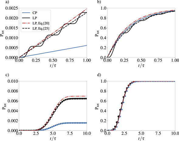
Figure 2. Temporal evolution of the probability for a high-energy photon with normalized energy γγ = ℏωγ /(me c2) = 103 to decay into an electron–positron pair while interacting with a plane wave background field in head-on collision. Considering a constant background field envelop with (a) a0 ≃ 82 corresponding to χ0 = 0.5 and (b) a0 ≃ 660 corresponding to χ0 = 4. Considering a background field with sin2 temporal profile with maximum field amplitude (c) a0 ≃ 82 corresponding to χ0 = 0.5, (d) a0 ≃ 660 corresponding to χ0 = 4. Solid lines correspond to the exact probability obtained by integrating numerically equation (9), dashed lines and dots to the theoretical prediction obtained from equation (25), for LP (ɛ = 0, black) and CP (ɛ = ±1, blue) cases. The red dash-dotted lines correspond to the theoretical prediction from equation (25) using the approximation of equation (20) for LP.
Download figure:
Standard image High-resolution imageIn all panels, the solid lines denote the exact probability computed by numerically integrating equation (9), considering either LP (black lines) or CP (blue lines) background field. We can see that, for χ0 = 0.5, CP produces less pairs than LP, while for χ0 = 4 CP is slightly more efficient (the difference between the two polarizations will be discussed in details in section 2.3.1). These probabilities are compared against the prediction of equation (25), computed using either the numerically evaluated  (dashed lines in panels (a) and (b), dots in panels (c) and (d)) or the approximation given by equation (20) to compute Rm
(red dot-dashed lines, only computed for LP as it is exact for CP). Note that here and in the following, whenever equation (20) is used, the improved Erber approximation equation (4) is exploited.
(dashed lines in panels (a) and (b), dots in panels (c) and (d)) or the approximation given by equation (20) to compute Rm
(red dot-dashed lines, only computed for LP as it is exact for CP). Note that here and in the following, whenever equation (20) is used, the improved Erber approximation equation (4) is exploited.
Panels (a) and (b) show an excellent agreement between the exact computations (solid lines) and equation (25) (dashed lines), both using the numerically integrated values of  . A remarkably good agreement is also found when considering the fully analytical approximation of equation (20) for
  (red dot-dashed lines). The probability is slightly overestimated in this case, as expected for χ0 ∼ 1 for which equation (20) shows the greatest departure from the exact expression of
  .
.
Similarly, an excellent agreement between all three approaches is found in panels (c) and (d) considering a short (5τ FWHM in intensity) background field. In this case the value of Rm
in each τ/4 interval is computed by taking the value of  given by the local maximum of the field, i.e. the time variation of the envelope is considered slow during τ/4. The validity of this assumption is confirmed by PIC simulations discussed in the following. In particular, figure 2 shows that the approach leading to the derivation of equation (25), which consists in treating the cumulative contributions of successive maxima of the background field, remains a very good approach even for ultra-short, few cycle, background fields.
Last, we note that the results of 1D PIC simulations performed with Smilei (see appendix
2.3. Guidelines for pair production optimizations
2.3.1. Influence of the background field polarization
Interesting insights into the role of the background field polarization on pair production can be gained from the asymptotic behavior provided by equations (22) and (23).
We recall that, motivated by experimental constraints, we compare LP and CP at fixed energy: this condition implies that the CP beam has a lower maximum amplitude. Because of this, for χ0 ≪ 1, equation (22) shows that any departure from the LP case leads to a tremendous decrease of  . Indeed the exponential cut-off of the pair production rate is strongly affected by the decrease of χm
with |ɛ| as shown in equation (14). In contrast, for χ0 ≫ 1,
. Indeed the exponential cut-off of the pair production rate is strongly affected by the decrease of χm
with |ɛ| as shown in equation (14). In contrast, for χ0 ≫ 1,  is an increasing function of |ɛ|: the reduction of the field peak amplitude is compensated by the fact that the absolute value of the amplitude is not time dependent (see equation (15)). Hence, in this range, increasing the background field ellipticity increases the pair production rate. However, the rate increase from the LP to the CP case is small (less than 12%), and it is thus of marginal use to consider CP for boosting pair production
7
.
is an increasing function of |ɛ|: the reduction of the field peak amplitude is compensated by the fact that the absolute value of the amplitude is not time dependent (see equation (15)). Hence, in this range, increasing the background field ellipticity increases the pair production rate. However, the rate increase from the LP to the CP case is small (less than 12%), and it is thus of marginal use to consider CP for boosting pair production
7
.
The differences between the LP and CP cases are clearly shown in the inset in figure 1(b), where  is found to be orders of magnitude larger than
  for χ0 ≪ 1 while
  is only about 10% larger than
  for χ0 ≫ 1. Similar conclusions can be drawn from figure 2. For small values of the photon parameter, χ0 = 0.5 (left panels), the pair production probability is significantly larger considering a LP background field instead of a CP one. For the higher value of χ0 = 4 (right panels), CP increases, but only marginally, pair production. For this reason, we will from now on focus on LP background fields, unless otherwise specified.
2.3.2. Influence of the background field amplitude and gamma-photon energy
The relative influence on pair production of the photon energy γγ
and the background field amplitude a0 (or equivalently intensity I0, as we consider here a given background field wavelength λ = 0.8 μm), is summarized in figure 3. It shows the probability Pm
for a high-energy photon to decay in a pair after crossing half a wavelength of a LP background field: (a) integrating numerically equation (17) which provides an exact value of Pm
; (b) using the approximate but fully analytical expression given by equation (20); (c) extracted from 1D PIC simulations of the interaction of a flash of high-energy photons colliding head-on with a plane wave (details are given in appendix
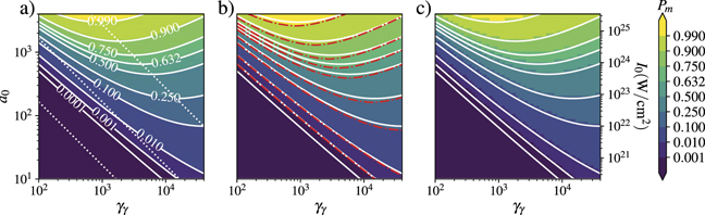
Figure 3. Probability Pm for a high-energy photon to decay into an electron–positron pair after crossing half-a-wavelength of a LP background field, as a function of the photon energy γγ = ℏωγ /(me c2) and background field amplitude a0: (a) integrating numerically equation (17), (b) computed using the approximate expression equation (20), (c) extracted from one-dimensional PIC simulations. In all three panels, the solid white lines report the isocontours of the first panel. In panel (b), the isocontours obtained from equation (20) are shown in red dot-dashed lines. White dotted lines correspond to constant values of χ0 = 0.1, 1, 16.5 from bottom left to top right corners.
Download figure:
Standard image High-resolution imageLet us first discuss panel (a) and note that, in addition to the probability isocontours (solid white lines), the dotted white lines represent the contours of constant quantum parameter, χ0 = 0.1, 1 and 16.5. As χ0 ∝ γγ a0, these are straight lines with a −45° inclination.
In the limit χ0 ≪ 1, i.e. the bottom-left of figure 3, Pm
assumes very small values. In this limit, the time-integrated rate Rm
τ/4 scales as ![${\gamma }_{\gamma }^{-1}{\chi }_{0}^{3/2}\enspace \mathrm{exp} \left[-8/(3{\chi }_{0})\right]$](https://content.cld.iop.org/journals/1367-2630/23/8/085006/revision2/njpac1975ieqn32.gif) (equation (22)) and the exponential term, depending only on χ0, gives the dominating contribution to Pm
. As a result, the isocontours of Pm
(solid white lines) behave as nearly straight lines, roughly parallel to the contours of constant χ0. We wish to stress however that the dependence on
(equation (22)) and the exponential term, depending only on χ0, gives the dominating contribution to Pm
. As a result, the isocontours of Pm
(solid white lines) behave as nearly straight lines, roughly parallel to the contours of constant χ0. We wish to stress however that the dependence on  cannot be fully ignored: the isocontours of Pm
are less steep than the isocontours of χ0 which indicates that Pm
increases faster with a0 than with γγ
. In this range of small χ0, for which probability and time-integrated rate are equivalent, the importance of increasing a0 to improve pair production was already pointed out in [36]. However, the probability variation with both a0 and γγ
needs to be examined in more details at higher χ0.
cannot be fully ignored: the isocontours of Pm
are less steep than the isocontours of χ0 which indicates that Pm
increases faster with a0 than with γγ
. In this range of small χ0, for which probability and time-integrated rate are equivalent, the importance of increasing a0 to improve pair production was already pointed out in [36]. However, the probability variation with both a0 and γγ
needs to be examined in more details at higher χ0.
Indeed, the dependence with  plays a more important role as χ0 increases so that χ0 cannot be considered as the only relevant parameter in order to optimize the pair production rate. This is clearly seen by considering the isocontours of Pm
in (a0, γγ
)-plane, figure 3(a): the isocontour slope becomes shallow and eventually changes sign. Thus, for any value of Pm
, a minimum field strength a0 is needed in order to obtain the desired level of probability. A corollary is that, at constant a0, increasing γγ
increases the probability Pm
up to a maximum value, beyond which a further increase of γγ
would only decrease Pm
. The minimum of each isocontour can thus be found by solving ∂Pm
/∂γγ
= 0, which one can recast in the form
plays a more important role as χ0 increases so that χ0 cannot be considered as the only relevant parameter in order to optimize the pair production rate. This is clearly seen by considering the isocontours of Pm
in (a0, γγ
)-plane, figure 3(a): the isocontour slope becomes shallow and eventually changes sign. Thus, for any value of Pm
, a minimum field strength a0 is needed in order to obtain the desired level of probability. A corollary is that, at constant a0, increasing γγ
increases the probability Pm
up to a maximum value, beyond which a further increase of γγ
would only decrease Pm
. The minimum of each isocontour can thus be found by solving ∂Pm
/∂γγ
= 0, which one can recast in the form

Interestingly, this equation involves only χ0 so that the minima of the probability isocontours lie on a straight line of constant χ0. This a priori surprising result can be better understood noting that both a0 and Pm are Lorentz invariants, the minimum value of a0 to reach a given probability Pm can depend only on the Lorentz invariant involving the photon energy, i.e. χ0. Solving numerically equation (26) for ɛ = 0 (LP case), we obtain 8 χ0 ≃ 16.5, which is reported by a dotted line in figure 3.
To conclude with figure 3, let us now turn to panels (b) and (c). Panel (b) reports the probability Pm computed from equation (20) and the corresponding isocontours (red dashed lines). Superimposing the isocontours (white lines) of the probability from panel (a), we can see an excellent agreement between the two approaches. This validates the approximate form, equation (20), which has the advantage to be completely analytical and can now be used to get quick yet precise estimates of the probability Pm . Last, panel (c) reports the probability extracted from 1D PIC simulations of the head-on collision of a flash of high-energy photons with a laser beam. The probability was extracted from the depletion of high-energy photons after crossing half a laser wavelength. Here again, a very good agreement is observed with the isocontours (white lines) obtained from the exact integration shown in panel (a). This last panel thus provides a cross-benchmark of our model and the Monte-Carlo module for nonlinear Breit–Wheeler pair production implemented in our PIC code SMILEI.
Our model can be used to predict the effectiveness of pair production for a given set of laser and high-energy photon parameters 9 . Most of the photons crossing the laser will be converted in pairs over a time Δt if the quantity RΔt in equation (25) becomes of order 1, for which 10 Ptot(Δt) ⩾ 0.63. In figure 4, we highlight in yellow the region in the (a0, γγ )-plane where the probability for a high-energy photon to decay into a pair after interacting with a single maximum (half-wavelength) of the laser pulse Ptot(τ/4) is equal or larger than 0.63 (the pulse duration is here τ/2, but the time required for the photon to explore half the laser wavelength is Δt = τ/4). The condition Ptot(Δt) = 0.63 is also shown for pulses with a step-like time profile (solid lines) and duration 5τ (green, Δt = 2.5τ) or 100τ (blue, Δt = 50τ), and pulses with a sin2 intensity time profile with FWHM 5τ (green dashed line, Δt = 5τ) and 100τ (blue dashed line, Δt = 100τ). Note that both step-like and sin2 time profiles correspond to laser pulses with the same energy and peak power, and lead to similar requirements to reach Ptot ≃ 0.63. Comparing the blue and green lines, we see that at constant γγ a longer pulse satisfies the condition of efficient conversion for a lower value of a0. Hence, even though the condition Rτ/4 = 1 (yellow solid line) is quite stringent and achieving a high probability level over a time interval τ/4 can be difficult, the condition RΔt ≳ 1 is significantly relaxed considering longer interaction time. Indeed, significant (order 1) pair production probability is expected on forthcoming multi-PW laser facilities (see section 4 for details).
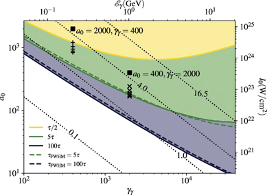
Figure 4. Position in the (γγ
, a0)-plane [equivalently in the ( )-plane] at which RΔt = 1 [Ptot(Δt) ≃ 0.63] for the interaction with a single maximum of the incoming pulse (half-wavelength, i.e. pulse duration equal to τ/2) for which the interaction lasts for Δt = τ/4 (yellow line) and for the interaction with pulses with a step-like time profile (solid lines) of duration 5τ (green) and 100τ (blue), and pulses with a sin2 time envelope with FWHM of 5τ (green dashed line) and 100τ (blue dashed line). The color-shaded areas above the plain lines correspond to RΔt > 1 (considering the step-like time profiles). The dotted black lines correspond to constant χ0 = 0.1, 1, 4, 16.5. The symbols highlight the parameters of the simulations discussed in sections 3.4 and 3.5.
Download figure:
Standard image High-resolution imageLet us also note that, when Rτ/4 ⩾ 1 (yellow area), more than 63% of conversion is achieved after crossing a single wavelength of the background field, and more than 99% of the incident gamma photons are converted into pairs in less than 3 periods. This gives a very robust condition for abundant pair creation, and it determines a limit above which is not useful to further increase the laser amplitude to increase the number of primary pairs. As we will show in the following, this condition (R τ/4 ⩾ 1) can also be invoked to find the optimal laser transverse shape and focal spot for a given laser energy. Indeed 3D PIC simulations, shown by the symbols in figure 4 and discussed in detail in the next section 3, show a different behaviour depending on whether their initial parameters lie in the yellow or green region of figure 4. In the case of the two simulations reported as squares in the figure, we will see that these differences are observed even though the simulation parameters correspond to the same value of χ0.
As a final remark, we point out that the probabilities considered so far are computed considering a given high-energy photon energy. In practice, we expect the high-energy photon beam to have a broad energy spectrum or at least a finite energy width (see e.g. references [25, 32, 39–46]). Accounting for such energy distributions is however straightforward as there is no coherence effects between the high-energy photons. The total probabilities can thus be computed independently for all relevant high-energy photon energies so that Ptot(γγ ) is actually a function of γγ . As an example, to compute the total number Npair of produced pairs, one only needs to integrate over the whole high-energy photon spectrum: Npair = ∫dγγ Ptot(γγ )dNγ /dγγ , where dNγ /dγγ denotes the high-energy photon energy distribution.
3. Geometrical effects on pair production: the case of LG beams
This section aims to generalize the model developed in section 2.2.2, to overcome the plane wave approximation and account for the laser beam transverse profile. We start by reminding some properties of the LG beams, limiting ourselves to the critical aspects for the understanding of pair production. We then compare the predictions of our theoretical model (generalized to account for the laser transverse profile in section 3.3) with the results of 3D PIC simulations, whose initialization is discussed in section 3.2. A thorough comparison of the efficiency of pair production considering beams with the same energy and different field structures is presented in sections 3.4 and 3.5. We explore first the impact of the beam geometry and amplitude in a regime of efficient pair production (time-integrated rate Rm τ/4 > 1) and then in a regime (Rm τ/4 < 1) more relevant for current experimental facilities (as will be discussed in the following section 4). Finally in section 3.6, we discuss some properties of the produced pairs, such as the energy spectrum and the propagation direction.
3.1. Properties of LG beams
The LG modes are solutions of the paraxial equation with cylindrical symmetry and a generalization of the Gaussian beam. Each mode is indexed by two integers: p ⩾ 0 for the radial order and ℓ for the azimuthal one. Hence, the notation LGpℓ will be used in the following to identify a specific mode.
Starting from equation (10), the electric field of an LG beam can be expressed using  , where the complex envelope upℓ
in cylindrical coordinates is [64]
, where the complex envelope upℓ
in cylindrical coordinates is [64]

where  is a normalization constant,
  are the generalized Laguerre polynomials,
  is the beam waist with w0 = w(z = 0) the waist at focus and
  the Rayleigh length, and
  is the generalized Gouy phase. Note that the LG modes described by equation (27) have all the same energy and that LG00 corresponds to a Gaussian beam with maximum field amplitude a0.
In order to infer how the structure of the LG modes might affect pair production we show in figures 5(a)–(d) the quantum photon parameter χγ for the head-on collision of photons of energy γγ = 400 with a LP LG beam at focus (i.e. z = 0) with a0 = 2000, p = 0 and ℓ ∈ [0, 3]. As can be seen in figures 5(a)–(d), for ℓ ≠ 0 the maximum of the field, and thus the peak values of the quantum parameter, are no longer along the beam axis (i.e. x = y = 0), in contrast with the Gaussian beam case. The radius at which the field has its maximum amplitude ρmax can be obtained by solving ∂ρ |upℓ |2 = 0, leading to:

with δij
the Kronecker delta. For p = 0, equation (28) can be solved analytically and gives  . While the radial position of the field maximum for p = 0 increases with |ℓ|, the amplitude decreases, as shown in figure 5(e), and tends asymptotically to zero for |ℓ| ≫ 1 as |2πℓ|−1/4. The maximum amplitude of the envelope u0ℓ
can be computed inserting ρmax into equation (27), which gives
. While the radial position of the field maximum for p = 0 increases with |ℓ|, the amplitude decreases, as shown in figure 5(e), and tends asymptotically to zero for |ℓ| ≫ 1 as |2πℓ|−1/4. The maximum amplitude of the envelope u0ℓ
can be computed inserting ρmax into equation (27), which gives

Figure 5(e) also shows  for p ≠ 0, obtained by inserting the numerical solution of equation (28) into equation (27). The maximum field amplitude for the LG beams decreases with both |ℓ| and p, and as a consequence the same behaviour is observed for the maximum value of χγ
(see figures 5(a)–(d)). Therefore, in the following we will consider only |ℓ| ⩽ 5 and p = 0, because of the higher field amplitude (hence higher values of χγ
) and because of the practical challenges in producing high order modes at relativistic intensity.
for p ≠ 0, obtained by inserting the numerical solution of equation (28) into equation (27). The maximum field amplitude for the LG beams decreases with both |ℓ| and p, and as a consequence the same behaviour is observed for the maximum value of χγ
(see figures 5(a)–(d)). Therefore, in the following we will consider only |ℓ| ⩽ 5 and p = 0, because of the higher field amplitude (hence higher values of χγ
) and because of the practical challenges in producing high order modes at relativistic intensity.
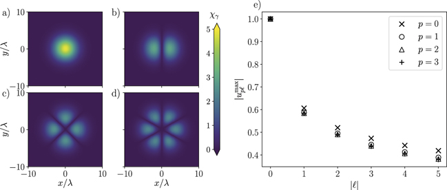
Figure 5. Photon quantum parameter χγ
in the head-on collision of photons of energy γγ
= 400 with a LP LG beam at focus (i.e. z = 0 in equation (27)) with a0 = 2000, p = 0 and (a) ℓ = 0, (b) ℓ = 1, (c) ℓ = 2, (d) ℓ = 3. (e) Maximum of the complex envelope  from equation (29) (black line) and for p ∈ [0, 3] as a function of |ℓ|. For p ≠ 0, equation (28) is solved numerically.
Download figure:
Standard image High-resolution imageNote that in the considered cases with ℓ ≠ 0, χγ has 2|ℓ| maxima in the transverse plane (see figures 5(b)–(d)) and, looking at the evolution in time, each maximum makes a full rotation around the laser propagation axis in |ℓ|τ. This means that, in a fixed transverse plane, a maximum rotates to the location of the next one in half a period.
If we consider the head-on collision of the LG beam with a gamma photon, the photon is crossing half a period of the field in τ/4. Hence, the photon crosses a rotating local maximum in τ/4. This observation is fundamental for generalization of the reduced model presented in the previous section 2.2.2, where we consider subsequent intervals of duration τ/4 to infer the total probability.
As noted in figure 5, the LG beams not only have a non-trivial spatial distribution of the fields in the transverse plane, but also a maximum field amplitude decreasing with |ℓ| (following equation (29)). In order to distinguish the impact on pair production of these two aspects, we discuss the interaction with extended Gaussian (EG) beams. For each LG beam (i.e. each value of |ℓ|), we define the associated EG beam as the Gaussian beam that has the same maximum field amplitude and carries the same total energy. As  decreases with |ℓ| (equation (29)) and the energy is kept constant, the waist of the EG beams increases with respect to the fundamental Gaussian (equivalent to LG00) as
  .
.
3.2. Simulation set-up
In what follows, we present 3D PIC simulations performed with the open-source code SMILEI [54], considering the setup schematically represented in figure 6. Each simulation reproduces a volume of 40λ × 40λ × 14λ (in the x, y and z directions, respectively) with spatial resolution λ/24 and temporal resolution at 95% of the CFL condition [65].

Figure 6. Typical set-up of the 3D PIC simulations, with λ and τ the laser wavelength and the optical cycle, respectively.
Download figure:
Standard image High-resolution imageAn intense laser pulse (with wavelength λ = 0.8 μm) is injected from the left boundary z = −5λ using the method presented in reference [66] that allows for the Maxwell-consistent injection of an electromagnetic wave with an arbitrary spatio-temporal profile. Here, this method is used to inject the laser pulse by prescribing its spatio-temporal profile in its focal plane [i.e. the (x, y)-plane at z = 0], as given by the real part of equation (27) at z = 0, multiplied by a temporal envelope so that the laser pulse has a sin2 temporal profile in intensity with FWHM τFWHM = 5τ, and total duration of 10τ. The laser beam collides head-on with a counter-propagating flash of high-energy photons with a finite longitudinal extension Lγ
= λ/6, transverse extension equal to the simulation box, and a density nγ
equal to the critical density nc = 0
me
ω2/e2. The duration of the simulation is long enough for the two light beams to stop interacting, but short enough so that none of the photons or secondary particles escape from the simulation box. All results presented hereafter have been extracted at the end of the simulations.
In sections 3.4 and 3.5, we present two series of simulations: the first one with a0 = 2000 and γγ = 400, the second with a0 = 400 and γγ = 2000, both series corresponding to a reference quantum parameter χ0 ≃ 6 × 10⁻⁶ a0 γγ ∼ 4.85 (for λ = 0.8 μm). For each series, we varied the transverse spatial profile of the high-intensity laser pulse in order to study the impact of the spatio-temporal field profile, comparing different LG beams (varying ℓ, but keeping p = 0) and the corresponding EG beams. Note however that within each series, a0 is left unchanged and refers to the maximum field amplitude of the reference Gaussian beam (for which we consider w0 = 3λ). As a result, within each set of simulations, the laser pulse energy is unchanged, equal to ≃10 kJ for a0 = 2000 and ≃410 J for a0 = 400. Conversely, the photon flash surface energy density me c2 γγ nγ d is ≃ 5 mJ/λ2 for the first series (with γγ = 400) and ≃25 mJ/λ2 for the second one (γγ = 2000).
As highlighted in figure 4 (squares), the reference Gaussian case of the first series of simulations allows us to explore the physics in the regime of high pair production probability after a single τ/4 interval (i.e. Rm τ/4 > 1, yellow region). On the contrary, with the second series we investigate a regime where efficient pair production is achieved thanks to the cumulative effects of several wavelength (i.e. Rm τ/4 < 1, but the reference Gaussian case is still above the green line in figure 4).
3.3. Reduced model for pair creation with arbitrary spatio-temporal laser beam profiles
In this section we generalize the model developed in section 2.2.2 to accurately describe pair production from complex, spatially structured laser beams.
To do so, we exploit the fact that we are here dealing with high-energy photons colliding head-on with the strong background field. Hence, the photon momenta are left unchanged as the photon crosses the background field, and their trajectories are straight lines so that the field seen by a given photon along its trajectory is known and depends only on the photon initial position (x0, y0) in the plane transverse to the direction of propagation of both light beams 11 . It follows that the quantum parameter of any photon is known throughout the photon interaction with the background field, and for a given background field, is determined uniquely by the photon initial position (x0, y0). As a result, the total probability Ptot for any photon to decay into a pair after interacting with the laser pulse is also determined by the photon initial position, and the total number of produced pairs at the end of the interaction between the flash of high-energy photons (with density nγ and longitudinal width Lγ ) simply reads

A key quantity to model pair production is thus the total cross-section σtot, here defined as the integral of the total probability over the transverse plane.
Notice that, as discussed in the last paragraph of section 2, for a given gamma photon spectrum σtot can be considered a function of γγ , and the total number of produced pairs can be computed integrating over the incident high-energy photon spectrum. Moreover, equation (30) can be easily generalised to account for a transverse profile of the incident high-energy photon beam. In particular, in the limit where this beam is much narrower than the laser beam, equation (30) reduces to σtot ≃ σγ Ptot, where σγ is the transverse area of the high-energy photon beam, and Ptot is computed at the (transverse) location of the high-energy photon beam.
To compute the total probability at any position (x0, y0) we use equation (25) and proceed as described in section 2.2.2, reconstructing the total probability from successive time intervals of duration τ/4 (as discussed in section 3.1, a photon at any position in the transverse plane explores in τ/4 a local maximum of the field amplitude whatever value ℓ assumes). One then only needs to compute the maximum field amplitude satisfactorily. For simplicity, we do so measuring the field amplitude at focus, taking the absolute value of the field envelope from equation (27) at z = 0. This approach, which neglects the effects of diffraction, is justified whenever the duration of the interaction (∼τFWHM) does not exceed the time zR/c for light to cross the laser pulse Rayleigh length. As shown in the following, this approximation proves satisfactory considering typical ultra-short (Ti:sapphire) light pulses.
The result of this procedure is shown in figure 7(a) for the case of a LG beam with ℓ = 5, p = 0 and a0 = 2000 colliding with a flash of photons with energy γγ = 400 (corresponding to χ0 = 4.85; all other parameters are specified in section 3.2). Panel (a) shows a map, in the transverse plane, of the probability Ptot computed over the whole interaction time in the transverse plane. Integrating over the transverse plane provides the measure of the total cross-section σtot ≃ 91.4λ2.
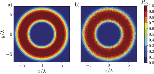
Figure 7. Probability map for a photon with energy γγ = 400 to produce a pair during the interaction with the LG05 beam with FWHM of 5τ and maximum amplitude of the reference Gaussian beam equal to a0 = 2000, corresponding to χ0 ≃ 4.85. (a) Analytical prediction from equation (25). (b) Numerical results from the 3D PIC simulation.
Download figure:
Standard image High-resolution imageTo test the impact of the approximations used in the model (phase and diffraction effects are neglected), we show in figure 7(b) the probability map extracted from a 3D PIC simulation, where all effects neglected in our model are taken into account. Here the probability is extracted at the end of the interaction as the ratio of the remaining photon linear density by the initial one. An excellent agreement is found with the theoretical prediction of panel (b), with a measured total cross-section σtot ≃ 91.0λ2, which confirms the predictive capability of our simple model for the case of spatially structured beams.
3.4. Simulations in the regime of high pair production probability (Rm τ/4 > 1)
In order to investigate the dependence on the laser structure of the number of produced pairs, we present here a study in the regime satisfying Rm τ/4 > 1 for the reference Gaussian beam, in which we expect efficient pair production. We remind that we consider here photons with normalized energy γγ = 400 and a reference Gaussian beam with maximum amplitude a0 = 2000, leading to χ0 ≃ 4.85 (all other parameters have been specified in section 3.2).
To test our analytical predictions and the assumptions at the base of our model, we performed simulations (hereafter referred to as frozen cases) in which the produced pairs are prevented to further radiate. In this condition, no secondary pairs are produced and the simulations allow to directly test the proposed analytical model. We also performed simulations including the full system dynamics (hereafter referred to as full cases), meaning that the produced pairs interact with the laser fields and potentially radiate. This allowed us to verify that we are still in the soft-shower regime, and that only a small departure from predicted number of produced pairs is indeed observed.
Figure 8(a) shows the number of produced pairs at the end of the interaction for all the tested cases, LP LG (in black), CP LG (blue) and EG (green), dots refer to the frozen simulations and squares to the full ones. Considering a LP LG laser beam, pair production efficiency increases with ℓ. This means that for the high value of a0 considered here, it is preferable to increase ℓ, even if it is decreasing the maximum amplitude (as shown in figure 5(e)), as it increases the characteristic transverse size of the beam, and so the interaction area where the probability is high (see inset in figure 8(a)). The EG beams (which have by construction the same maximum amplitude of the LG beams but Gaussian profile) are more efficient than the corresponding LG, up to ℓ = 4, as they have a bigger region with substantial probability in their probability maps. However, a slightly greater number of pairs are produced in the simulation with LG05 than EG05 beam. This because the maximum field amplitude has dropped substantially and a large part of the interaction region in the EG case has low probability of pair production (see inset in figure 8(a)). Predictions form our model discussed in section 3.3 and based on equation (30), shown in dashed lines, are in very good agreement with both EG and LG simulations.

Figure 8. (a) Number of produced pairs, and corresponding cross section σtot/λ2 after the interaction of gamma photons with energy γγ = 400 and a counter-propagating LG with p = 0, ℓ ∈ [[−1, 5]] and a0 = 2000 [CP (blue), LP (black)], and the corresponding LP EG (green). Frozen simulations (dots), full simulations (squares) and theoretical predictions from equation (30) (dashed lines). The insets show the probability map for the LG00, LG05 and EG05 cases. (b) Relative difference in the number of produced pairs between the frozen and full simulation results.
Download figure:
Standard image High-resolution imageBased on the prediction from figure 1, for the considered χ0 ≃ 4.85 we would expect at first look a higher efficiency in the CP case than with LP, contrary to what is obtained from PIC simulations (blue symbols in figure 8(a)). However, given the spatial structure of the laser field in the transverse plane, in a large part of the interaction region the quantum number is χ < 2.5, i.e. the value above which CP should be favoured based on the analysis shown in figure 1(b) obtained within the plane wave approximation. Hence, the slightly higher number of pairs produced in the CP case with respect to LP in the region where χ > 2.5, cannot compensate the higher efficiency of LP in the region of χ < 2.5. Note that the results using a CP beam are independent from the sign of ℓ (i.e. from the total angular momentum). This suggests that the total angular momentum of the laser has no effect on the number of pair produced. Note however that we do not account for the spin polarization effects. Since we are focusing on the soft shower regime where there are few secondary pairs, the dynamics of the pairs affected by spin effects is expected to play a minor role for pair production in our case. Moreover the dynamics of the produced pairs is not the main concern of this study. Nevertheless, in other configurations spin effects can impact the created pairs and gamma photons dynamics as shown in references [67, 68].
For completeness, we compare the results of the frozen cases with simulations reproducing the full dynamics of the system (squares in figure 8(a)). As highlighted in figure 8(b), the difference in the produced number of pairs is always below 25% of its value in the frozen case, and it decreases with |ℓ|. This confirms that the majority of pairs comes from the conversion of primary gamma photons and not from subsequent radiation, as expected for a soft-shower. In this regime, our model, which accurately captures the physics of pair production for the frozen simulations (dashed lines), can be therefore used to predict pair production in realistic conditions.
3.5. Simulations in the regime of moderate pair production probability (Rm τ/4 < 1)
In this second series of simulations we explore the regime of Rm τ/4 < 1, maintaining the same maximum χ0 as in the previous section by exchanging the values of field amplitude (now equal to a0 = 400) and photons energy (now equal to γγ = 2000). Note that considering a laser duration (τFWHM = 5τ), we still expect efficient pair production (the reference plane wave simulation lies above the green dashed line in figure 4). This can be seen in the inset of figure 9(a) for the Gaussian case LG00 where a significant region exhibits a probability of order 1.

Figure 9. (a) Number of produced pairs and corresponding cross section σtot/λ2, after the interaction of gamma photons of energy γγ = 2000 with a counter-propagating LG beam with p = 0, ℓ ∈ [[−1, 5]] and a0 = 400 [CP (blue) and LP (black)], and the corresponding LP EG (green). Full simulations (squares) and theoretical predictions from equation (30) (dashed lines). The insets show the probability map for the LG00, LG05 and EG05 cases. (b) Relative difference in the number of produced pairs between the frozen and full simulation results. The frozen cases are not shown in panel (a) as the difference with the full ones is always below 15%.
Download figure:
Standard image High-resolution imageAs figure 9 shows, for the simulations with LG beams the number of produced pairs is optimized for ℓ = 3. The increase for |ℓ| ⩽ 3 can be explained as in the previous section by geometrical considerations, i.e. the area with the field being large enough to reach Ptot of order one is getting wider with |ℓ|. In the contrary for |ℓ| > 3, the laser field amplitude becomes too low and having a laser beam with a larger transverse extension does not improve pair production. This is due to the fact that the field is becoming too low, so that the effect of decreasing Ptot on pair production is more important, and is not compensated anymore by the increase in transverse size.
Moreover, in this regime, all LG beams perform better than the corresponding EG, given that the region with high (even though smaller than in the previous section 3.4) probability is larger for the LG than EG, as shown in the inset of figure 9 for ℓ = 5. Also, a similar behaviour as discussed in the previous section 3.4 is observed for the CP simulations and can be explained with the same reasoning. Last but not least, our model is reproducing with high accuracy the observed number of pair in this case too.
3.6. Energy and angular distribution of the produced pairs
The energy-angular distribution of the produced pairs in the z–x plane (i.e. the plane formed by the laser propagation direction  and the polarization direction
  for the LP case) recorded at the end of the interaction is shown in figure 10 considering the reference LP and CP Gaussian beams. The top row gives the positron distribution in θ = arctan(px
/pz
) and in energy for the LP beams and the bottom one for the CP beams. The insets show the energy spectra of particles moving in the positive (same as the laser, black line) and negative (same as the gamma flash, red line) z-directions.
for the LP case) recorded at the end of the interaction is shown in figure 10 considering the reference LP and CP Gaussian beams. The top row gives the positron distribution in θ = arctan(px
/pz
) and in energy for the LP beams and the bottom one for the CP beams. The insets show the energy spectra of particles moving in the positive (same as the laser, black line) and negative (same as the gamma flash, red line) z-directions.

Figure 10. Positron distribution in Lorentz factor γ (equiv. normalized energy) and angle θ = arctan(px /pz ) for the first simulation series (left column) and for the second one (right column); LP (CP) in the top (bottom) row. The insets show the energy spectra for positrons propagating in the positive (black line) and in the negative (red line) directions.
Download figure:
Standard image High-resolution imageAt high a0 (panels (a) and (c)) the produced pairs, initially generated with momentum in the negative z-direction, are predominantly moving in the same direction as the laser (corresponding to θ = 0°) within a cone of aperture 40°, meaning that they have been slowed down and then pushed by the laser. They reach a maximum energy of ≃104 me c2 for the LP case and ≃8 × 10³ me c2 for the CP beam, consistent with the decrease of the peak field amplitude in CP with respect to LP at constant energy.
The spatial distribution is drastically modified when considering a0 = 400. Even if there still is a substantial amount of pairs propagating in the laser direction, the majority of them keep their original direction, along the initial gamma photons propagation axis and anti-parallel to the laser pulse one. For these pairs the maximum energy is independent from the polarization, as shown in figures 10(b)–(d), contrarily to the pairs that are slowed down and pushed by the laser (right side of the quadrants or black line in the insets).
This study, supported by complementary simulations (not shown), suggests that for a0 ≳ γγ most of the created particles will end up propagating along the laser direction, while for smaller values of the laser maximum amplitude a large fraction of pairs will keep their original direction. A complete characterisation of the pairs spectrum and directionality is beyond the scope of this work, and will be investigated in more details in the future, as it can give important information for the planning of upcoming experimental campaigns.
4. Discussion
The model developed in this work allows to predict the pair production capability of upcoming facilities. In figure 11, we discuss the pair production maximum probability and total cross-section as a function of the photon energy and laser amplitude. The considered parameter range is relevant to ultra-short Ti:sapphire (λ = 0.8 μm) lasers, where studies of high-field physics and QED are already planned [69–72]. Two types of facilities can be distinguished. First, the Apollon 12 , CoReLS 13 and ZEUS 14 facilities (shown in black in figure 11) are designed to deliver multiple light beams with duration in between 15 and 30 fs FWHM and peak power from 1 to 10 PW. Second, the FACET-II 15 and LUXE 16 experiments will couple conventional electron accelerators with high-intensity (100 TW-class) ultra-short laser pulses (in white in figure 11).
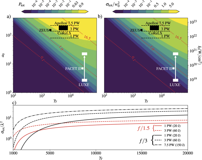
Figure 11. Model predictions considering a laser pulse with sin2 time-envelope in intensity (τFWHM = 25 fs) and λ = 0.8 μm. (a) Maximum pair production probability from equation (25). (b) Total cross section normalised to  using the model discussed in section 3.3. In both panels (a) and (b) the red lines denote contours of constant χ0 = 0.1, 1, 16.5. The regimes accessible with current and upcoming facilities are also reported. (c) Total cross section normalised to λ2 as a function of γγ
computed for the Apollon facility operating at 1 PW (solid lines), 3 PW (dashed lines) and 7.5 PW (dash-dotted line) and with focusing aperture f/3 (black lines) and f/1.5 (red lines). In this last panel, at a given power, the laser energy is the same for the different focusing aperture f/N.
using the model discussed in section 3.3. In both panels (a) and (b) the red lines denote contours of constant χ0 = 0.1, 1, 16.5. The regimes accessible with current and upcoming facilities are also reported. (c) Total cross section normalised to λ2 as a function of γγ
computed for the Apollon facility operating at 1 PW (solid lines), 3 PW (dashed lines) and 7.5 PW (dash-dotted line) and with focusing aperture f/3 (black lines) and f/1.5 (red lines). In this last panel, at a given power, the laser energy is the same for the different focusing aperture f/N.
Download figure:
Standard image High-resolution imageIn figures 11(a) and (b) the accessible a0 and typical γγ envisioned with these facilities (following the reference articles) are reported. For Apollon only, we computed a0 considering a 20 fs light pulse delivering 20, 60 and 150 J on target, corresponding to peak power of 1, 3 and 7.5 PW, respectively. The reported value of a0 is then computed for a LP Gaussian beam with focusing aperture f/3 (where the beam waist for a focusing aperture f/N is w0 ≃ 0.90Nλ ≃ 2.2 μm), using

Note in addition that, as most of these facilities will operate in the χ0 ≳ 1 regime, we report for the photon energy that of the electron beams either expected from laser-driven wakefield acceleration (for Apollon, CoReLS and ZEUS) or emerging from the linear accelerators (for FACET-II and LUXE). In the case of a broad (e.g. synchrotron-like) energy distribution for the high-energy photon source, the expected number of produced pairs can be computed integrating the reported values of Ptot or σtot over the full high-energy photon spectrum. As detailed below, this integration can be carried out in two rough but straightforward ways depending on the kind of facility (multi-PW or laser combined with a conventional accelerator) that is considered.
Let us now focus on panel (a), which shows the maximum total decay probability (from equation (25)) for a photon with energy γγ colliding head-on with a LP Gaussian laser pulse with maximum field strength a0 and duration τFWHM = 25 fs (typical for the facilities listed above). This panel suggests the strategy to optimize pair production depending on the type of facility.
First, despite the extremely high electron beam energies, facilities such as LUXE and FACET-II (in white in figure 11) offer the possibility to probe the regime of moderate quantum parameter (χ0 ≲ 1) for which pair production may be observed (Ptot ≃ 10−2) but will not be abundant. This limit might be overcome by increasing the laser power up to few 100's of TW (300 TW are envisioned at LUXE), which allows to enter the quantum regime (χ0 > 1) and increase Ptot to values exceeding 0.1. On these facilities however, because Ptot will not assume large values, increasing a0 (e.g. by focusing the laser pulse as much as technically possible) is one of the most promising path to achieve abundant pair production.
In contrast, provided that multi-GeV electron beams can be obtained from laser wakefield acceleration, abundant pair production (Ptot ≳ 0.63) is expected on all multi-PW laser facilities with the focalisation technique already in place (typically an aperture in between f/3 and f/4 was considered in figure 11).
Similar conclusions can be drawn from panel (b) where we examine in more details the influence of the laser pulse spatial profile, by looking at the total cross-section
17
σtot (as defined by equation (30)) normalized to  , considering a Gaussian laser beam with the same temporal properties as in panel (a).
For the FACET-II and LUXE facilities, the total cross-section assumes very small values but increases fast as a0 is increased: e.g. for LUXE, σtot increases by 3 orders of magnitude increasing a0 by a factor 10. Clearly, operating at large field strength will be a bottleneck for achieving abundant pair production on these facilities.
In contrast, in the range of parameters covered by multi-PW facilities, the dependence of σtot with a0 is much weaker. As in addition,  (consistent with Ptot ≃ 1 at the center of the beam), it becomes interesting for these facilities to increase the laser transverse size rather than opt for tight focusing.
Let us then discuss in more details the impact of focusing for the three upgrades of the Apollon facility (at 1, 3 and 7.5 PW). In panel (c), we present the total cross section (in units of λ−2) as a function of γγ , considering either the standard f/3 aperture (black lines) or the more challenging f/1.5 aperture (red lines). For each laser power, a tighter focusing reduces the beam waist but increases the maximum a0.
In all cases, the cross section is rapidly increasing with the photon energy for γγ ≲ 2 × 10³ (≃1 GeV). It is almost flat as γγ reaches 5 × 10³ (≃2.5 GeV), which suggests that it is not worth increasing the photon energy above this value in forthcoming experiments to optimize pair production in the soft-shower regime.
As shown in panel (c), for a given laser power the cross section for f/1.5 is larger than for f/3 only for small values of γγ , while the opposite behaviour is observed at large γγ (of the order of a few GeV). This means that such tight focus, which is technologically very challenging, is not necessary for pair creation in forthcoming experiments on Apollon.
To test this prediction, we have performed complementary 3D PIC simulations of the 3 PW case with f/3 and f/1.5 (a0 = 138.8 and 276.7, respectively) interacting with a gamma flash with energy γγ = 104. These simulations give σtot ≃ 26.8λ2 for f/3, which is indeed larger than the value σtot ≃ 19.5λ2 obtained for the tight-focusing f/1.5 case. These simulation results are consistent with our reduced model predictions, but also noticeably above its predictions, which are σtot ≃ 16.2λ2 for f/3 and σtot ≃ 6.5λ2 for f/1.5 (as given by figure 11(c)).
One of the reason of the discrepancy is that our calculations are performed at focus, neglecting diffraction. While this was a very good approximation for the parameters considered earlier (see section 3.3), it is not correct when considering tightly focused intense background fields and an interaction region larger than the Rayleigh length. The model can be easily generalized to include diffraction. Doing so improves our predictions to σtot ≃ 22.2λ2 for f/3 and σtot ≃ 9.8λ2 for f/1.5. These values are now significantly closer to our 3D PIC simulation results, and are also in excellent agreement (within 1%) with additional 3D PIC simulations in which secondary pair production is not accounted (frozen case). Secondary pairs, responsible for a further increase of about 20% for the f/3 case and by a factor ×2 for the tightly-focused f/1.5 case, are not included in the model and are the source of the remaining discrepancy. This suggests that for the highest peak intensity considered here we are at the limit of the soft-shower regime and the model should be considered as providing a lower bound estimate for pair production.
Let us finally briefly comment on how the effect of a broad energy spectrum and transverse extension of the high-energy photon beam can be accounted for depending on the type of facility considered.
In the case of FACET-II and LUXE facilities, both Ptot and σtot are very steep functions of γγ , e.g. increasing by several (more than 4) orders of magnitude for the FACET-II configuration as γγ is increased from 5 × 10³ to 3 × 10⁴. One can thus expect that, for these facilities, only the photons with the highest energy contribute to pair production. The total number of produced pairs can then be estimated considering only those photons with the highest energy (maximum γγ as reported on panels (a) and (b)). If the high-energy photon beam is much narrower that the laser beam, the total number of produced pair can be computed from the number of photons and Ptot evaluated at this maximum γγ . If instead the high-energy photon beam has a large transverse distribution, the final number of pairs can be calculated by taking the high-energy photon surface density and σtot computed at the maximum γγ .
For the multi-PW laser facilities, and large background field strength a0, we have seen that both Ptot and σtot (for the latest, see e.g. panel (c) for the Apollon facility) reach a plateau above a minimum value of the photon energy (e.g. γγ ≃ 5 × 10³ in the case of panel (c) discussed above). Hence, pair production will follow primarily from the decay of the high-energy photons in this plateau. A simple estimate of the number of produced pairs will then be obtained from either the number of all photons in the plateau region and a typical value of Ptot (if the photon beam transverse size is small with respect to the laser beam waist) or from their surface density and σtot obtained for this energy range (if the photon beam transverse size is large).
5. Conclusion
In summary, we have presented a systematic study of nonlinear Breit–Wheeler pair production in the head-on collision of high-energy gamma photons with an ultra-high intensity laser beam. Combining analytical modeling and PIC simulations embarking the relevant QED modules, we have evaluated the impact on the efficiency of pair production of the laser spatio-temporal profile (comparing e.g. Gaussian with different focal spots and LG pulses) and parameters such as polarization, intensity and duration. Motivated by experimental constraints, we have considered fixed laser energies while changing these parameters.
We have explored laser field strength and photon energy parameter ranges relevant for currently and/or upcoming high-power laser facilities, focusing in particular on ultra-short Ti:sapphire laser facilities. A reduced model was proposed that allows to describe pair production in the regime of soft-shower, where secondary pair production can be neglected. This model, that would in principle allow to predict a minimum number of produced pairs, is found to agree remarkably well with 3D PIC simulations over a broad range of parameters, highlighting the importance of the soft-shower regime for experiments on the forthcoming laser facilities.
The model also allows to distinguish two regimes of interaction depending on whether the probability for a photon to decay into a pair as it crosses a single half-wavelength of the laser pulse is large (of order 1) or not. The two regimes are not however fully determined by the photon maximum quantum parameter χ0, so that the laser field strength parameter a0 and photon energy γγ do not play a symmetric role in the system dynamics. This was confirmed in 3D PIC simulations where the two regimes were investigated at χ0 = 4.85 considering laser beams with complex spatio-temporal profiles, LG beams in particular, and different polarizations. It was found that, for a fixed laser energy, using circular polarization or LG does not improve significantly pair production. As they are also quite difficult to achieve experimentally, their effect on pair production is too marginal to be interesting for applications. It was found however that, in the regime of high pair production probability, it can be preferable not to focus much the laser beam (keeping the same total energy with lower peak intensity) and maintain a Gaussian shape in order to maximise the area with high-enough fields for efficient pair production.
These findings help to draw guidelines for future experiments on ultra-high intensity facilities. We show in particular that the path to abundant pair production is different whether one considers 100 TW-class or multi-PW laser systems. In particular, for facilities such as FACET-II or LUXE, 10 to 100 TW-class lasers will be coupled to ultra-relativistic 10–20 GeV electron beams emerging from conventional electron accelerators. On these facilities, pair production will develop in the low probability regime and operating in a tightly-focused configuration to access the highest possible laser field strength will be a major experimental challenge. In contrast, using multiple laser beam multi-PW facilities will operate in the regime of high pair production probability. In this regime, the pair production efficiency (measured in our work in terms of a total cross section) depends more strongly on the laser pulse transverse size than on its maximal field strength so that operating with standard (not too tight) focusing aperture increases the number of produced pairs. Interestingly, producing high-energy photons (or electrons, e.g. through laser wakefield acceleration) of a few (∼5) GeV shall be enough for these facilities as higher energies do no help increase significantly the pair production efficiency in this high probability regime.
To conclude, this work provides a deeper understanding of the optimal conditions for pair production in upcoming experimental campaigns exploring nonlinear Breit–Wheeler pair production. It focused on pair production seeded by high-energy photons, and it will be interesting for future works to investigate the differences with the case where ultra-relativistic electrons are used to seed the pair production process. Studying the transition from the soft-shower to the cascade/avalanche regime in which secondary pairs and radiations play a dominant role is another interesting perspective.
Acknowledgments
The authors are grateful to F Amiranoff, P Audebert, S Corde, L Gremillet, L Lancia, R Nuter and C Thaury for stimulating discussions. This work used the open-source PIC code SMILEI, the authors are grateful to all SMILEI contributors and to the SMILEI-dev team for its support. Simulations were performed on the Irene-Joliot-Curie machine hosted at TGCC, France, using High Performance Computing resources from GENCI-TGCC (Grant No. 2020-x2016057678). This publication is also supported by the Collaborative Research Centre 1225 funded by Deutsche Forschungsgemeinschaft (DFG, German Research Foundation)—Project-ID 273811115—SFB 1225.
Data availability statement
All data that support the findings of this study are included within the article (and any supplementary files).
Appendix A.: Approximation of 

In this appendix, we detail how the integral  (equation (19)) can be efficiently approximated by equation (20). To do so, let us start by stressing that, in general, and in particular at small χ, b0(χ) is a steep function of χ. One thus expects the principal contribution to the integral to come from the phase φ around φm
= π/2, for which χ0Ψɛ
(φ) ≃ χm
with
(equation (19)) can be efficiently approximated by equation (20). To do so, let us start by stressing that, in general, and in particular at small χ, b0(χ) is a steep function of χ. One thus expects the principal contribution to the integral to come from the phase φ around φm
= π/2, for which χ0Ψɛ
(φ) ≃ χm
with  . To compute the contribution of this maximum analytically, we approximate the integrand in equation (19) around ϕm
as
. To compute the contribution of this maximum analytically, we approximate the integrand in equation (19) around ϕm
as

where sɛ (χm ) is chosen so that the exact and approximated integrand have the same second derivative at φ = φm , which gives

With the ansatz equation (A.1), the integral can be performed analytically, leading to

The ansatz equation (A.1) gives a good approximation of the integrand for arbitrary values of ɛ as long as χm is small enough. It is also exact (for all χ0) in the cases ɛ = ±1 for which s±1(χm ) → +∞. Hence, equation (A.3) provides a very good, fully analytical approximation of equation (19) for a wide range of ɛ and χ0.
The approximation however needs to be corrected for χ0 ≫ 1 and |ɛ| < 1. In this limit, the integrand in equation (19) can be approximated using equation (6) leading to

Equations (A.3) and (A.4) can be combined in equation (20). This form ensures the correct asymptotic behaviour of the integral equation (19) in both small and large χ0 limits. It departs from the exact expression (integrated numerically) by less than 20%, the error being maximum for intermediate values of χ0 ∼ 1. This was tested over a broad range of χ0 ∈ [0.1, 1000] for various polarization parameter ɛ ∈ {0, 0.25, 0.5, 0.75, 1}.
Appendix B.: Details on 1D PIC simulations
A series of 1D3V (1 dimensional in space and 3 dimensional in velocity) PIC simulations, considering a plane wave colliding head-on with a flash of gamma photons, have been performed to produce figure 3(c). We simulated a box of length 2.5λ with spatial resolution λ/256, for a simulation time of 1.75τ, with temporal resolution τ/512. This is a long enough time to study the full interaction of the plane wave with a flash of gamma photons of extension λ/2 and extract the probability from the number of surviving photons. The probability map in figure 3(c) is obtained from the results of 4096 (64 × 64) simulations performed over a the logarithmically spaced range of a0 ∈ [10, 4000] and γγ ∈ [100, 40 000].
Footnotes
- 5
- 6
Throughout this paper, we consider background fields with a finite (e.g. sin2) temporal profile so that this time t0 is uniquely defined.
- 7
In particular as, in practice, implementing CP on multi-petawatt facilities would lead to a decrease of the delivered laser pulse energy.
- 8
Solving equation (26) for arbitrary values of ɛ ∈ [−1, 1] leads to χ0 in between 16.5 and 17.2, and corresponding values of Iɛ (χ0) in between 5.3 and 6.0.
- 9
In the case of large secondary pair production, our prediction will underestimate the number of pairs as our analysis is limited to the soft-shower regime.
- 10
Note that in this limit, the probability cannot be assimilated to the time-integrated rate, as in the case of very weak pair production.
- 11
For analytical tractability, we consider all photons to be propagating exactly in the z-direction.
- 12
- 13
CoReLS, in Gwanju, South Korea, is operating at up to 4PW [3]; see also the CoReLS website.
- 14
A 3PW laser facility being built at the University of Michigan; see the ZEUS website.
- 15
FACET-II is planned at SLAC National Accelerator Facility [74]; see also the FACET-II website.
- 16
LUXE is an experiment proposed at the European XFEL [75]; see also the LUXE experiment website.
- 17
Since the Gaussian field profiles depend on the transverse coordinate through the ratio ρ/w0 (equation (27)),
is independent of w0.
