


Abstract
Unambiguous determination of the electric field of arbitrary ultrashort pulses is the key for time and frequency standards, attosecond science, and precision spectroscopy. However, a single-step technique that can simultaneously and directly characterize the spectrum, spectral phase, and the carrier-envelope phase (CEP) information of an arbitrary ultrashort pulse remains elusive. This technological roadblock hinders the current field from studying non-repeating single-shot events, since ultrashort laser pulses are often unstable. Here, we introduce a single-step reference-free technique through polarization interfering electric field with phase inverted electric field (PIE-PIE) to directly measure arbitrary ultrashort pulses in single-shot operation without using any retrieval algorithm. PIE-PIE utilizes highly efficient spectral phase conjugation based on four-wave-mixing. The ability to fully determine the spectrum, spectral phase, and CEP of relatively low intensity single-shot pulses will revolutionize ultrafast sciences and enable studies of arbitrary non-repeating ultrafast events.
Export citation and abstract BibTeX RIS
1. Introduction
Today, ultrafast dynamic studies are routinely carried out with ultrashort femtosecond laser pulses. Therefore, a precise characterization of the electric field of these ultrashort pulses is the key to understanding and controlling various ultrafast phenomena, including chemical reactions, phase transition, electron and phonon dynamics, laser-matter interactions, biological processes, attosecond pulse generation, and time and frequencies standards [1–12]. The carrier-envelope phase (CEP), the relative phase between the carrier wave and pulse envelope, affects the carrier–envelope offset frequency, whose stabilization is critical for a range of ultrafast processes including time and frequencies standards, attosecond pulse generation, and precision spectroscopy [1, 2, 4, 5, 13]. Currently, however, no single-step reference-free technique can directly characterize the electric field and the CEP information of an ultrashort pulse in the visible and near IR without the need of any retrieval algorithm. The challenge comes from the fact that determining the electric field of ultrashort pulses precisely requires the measurements of the spectrum and spectral phase with CEP information at a single-shot operation, which is a long-standing challenge.
Currently, a full characterization of an arbitrary ultrashort pulse typically requires two sets of measurements, one providing the temporal characterization and the other carrier-envelope-phase characterization [11, 14, 15]. Frequency-resolved optical gating (FROG), a standard temporal measurement technique, measures the spectrally-resolved autocorrelation and requires a phase-retrieval algorithm [16–18]. Another standard temporal measurement technique, spectral phase interferometry for direct electric-field reconstruction (SPIDER), measures the slope of the spectral phase [19, 20]. Both FROG and SPIDER can measure the spectral phase, along with spectrum, at single shots but fail to yield any CEP information. CEP without spectral phase information can be determined at single shots using various techniques including the f-to-2f interferometer, and above-threshold ionization measurements [21–24]. The f-to-2f interferometer determines the carrier-envelope offset frequency by measuring the beat note between the frequency-doubled lower-frequency end of the comb spectrum with the higher-frequency end of the fundamental comb spectrum [21]. The above-threshold ionization measurements can reveal CEP by detecting asymmetric spectra of the scattered electrons with two detectors located at the opposite ends of an experimental vacuum system [22, 23]. These techniques, however, yield no precise information on the spectral phase.
An ultrashort pulse may be characterized using a single-device technique of electro-optic samplings [25] or attosecond streaking [26], but each suffering severe limitations. Electro-optic samplings require a reference pulse shorter than the period of the electric field to be characterized and rely on the Pockels effect [25, 27]. Therefore, the technique is limited to a rather long wavelength region from terahertz to mid-infrared, where the assumption of a flat frequency response is appropriate [25]. This assumption requires the condition that the spectrum of the pulse lies below the first phonon resonance of the sensor crystal [25]. Electro-optic samplings can also be combined with FROG, a technique called FROG capable of CEP determination (FROG-CEP) [27], to characterize wavelength regions shorter than terahertz, but it still requires a part of the spectrum to satisfy the conditions mentioned above [27]. Attosecond streaking requires the test pulse to have an appropriate shape and high enough intensity to generate a single extreme-ultraviolet attosecond pulse [26, 27]. Therefore, a single-step technique that can fully characterize an arbitrary ultrashort pulse with CEP information remains elusive.
Here, we propose a simple single-step technique through polarization interfering electric field with phase inverted electric field (PIE-PIE) to directly measure the frequency domain electric field E(ω). PIE-PIE can determine the electric field with the CEP information in real-time for individual ultrashort pulses, a quest that has never been achieved. Moreover, our technique is reference-free, only requires relatively low power, and the characterization is direct without any retrieval algorithm. This PIE-PIE technique relies on phase conjugation. Phase conjugation has a range of applications including correcting aberration, cascade lasers, and all order temporal distortion correction [28–31]. The implementations of spectral phase conjugation for ultrashort pulses have been done using techniques such as time lens [32], photon echo [33, 34], spectral hole burning holography [35], and wave mixing of spectrally decomposed waves [36]. However, phase conjugation has never been explored for ultrashort pulse characterization. Here, for the first time, we apply the phase conjugation for ultrashort pulse characterization. The ability to measure spectrum and spectral phase with CEP information of relatively low power non-repeating ultrashort events will advance ultrafast metrology and enable a broad range of applications.
2. Direct measurement of electric field
We propose a very simple concept of PIE-PIE to directly measure the frequency domain electric field E(ω). The technique simultaneously measures the spectrum and spectral phase with CEP information. The CEP continuously changes as a pulse travels through a dispersive medium, caused by the difference between the group and phase velocity of the dispersive medium (See appendix

Figure 1. Schematic and principles of the PIE-PIE device for direct determination of the spectrum, spectral phase, and CEP of a single ultrashort pulse (a) the single-step flow chart of the PIE-PIE technique assuming an ideal spectral phase conjugation. The unknown pulse and its phase conjugation are superimposed in orthogonal polarization. The superposition allows the spectrum, spectral phase, and CEP to be extracted from the spectrally-resolved polarization state measurement. (b) Schematic diagram of the experimental setup. (c) Schematic diagram of an example of a spectrally-resolved polarimeter using common off-the-shelf optical elements. BS—50:50 beam splitter, PBS—polarizing beam splitter, HWP—half-wave plate, QWP—quarter-wave plate, D—detector (spectrometer).
Download figure:
Standard image High-resolution imageThe schematic of the proposed PIE-PIE setup is shown in figure 1(b). An unknown ultrashort pulse E(ω) with 45° linear polarization is first heavily attenuated to avoid saturation of the spectrometers and unwanted non-linear effects in the ensuing beam lines. Attenuator such as a thin-film-based broadband attenuating mirror [37] can be used since the reflected pulse retains near identical spectral phase, although preserving the spectral phase is not a requirement for an accurate measurement. Next, the pulse enters the PIE-PIE device, where an interferometer splits the incident beam into horizontal and vertical components. The horizontal component is phase conjugated and later recombined with the vertical component at the output. The input polarization can be adjusted using a half-wave plate to vary the split ratio and route more power to the phase conjugation arm if its efficiency is low. As this phase conjugation process requires real-time spectral phase conjugation, the time lens technique [32] is a preferred method since it is real-time and also reference-free. Methods based on switchable photonic-crystal mirror [38] and dynamic photonic structures via Bloch oscillations [39] have also been proposed for phase conjugation of ultrashort pulses. The output of the interferometer is measured by a spectrally-resolved polarimeter. This spectrally-resolved polarization measurement is where the core concept of PIE-PIE comes into play. The concept of PIE-PIE is to determine the spectral phase between the original electric field and the phase conjugated field by superimposing them in orthogonal polarization and measuring the spectrally-resolved polarization state (see figure 1(a)), which can be written as

where jout(ω) is the Jones vector describing the angular frequency component ω of the recombined beam, ϕ(ω) is the spectral phase of the original electric field, H(ω) is the frequency dependent transfer function of the phase conjugation process and contains the dispersion mismatch between the two interferometer arms, and τ is the delay time between the two interferometer arms. The transfer function induces an additional spectral phase and attenuation to the beam depending on the phase conjugation mechanism and its efficiency. An ideal phase conjugation process has a unity transfer function of H(ω) = 1. Please note that any dispersion mismatch of the spectral phase acquired in the two arms is embedded into this transfer function for simplicity. In fact, the exponential term with the delay time exp(iωτ) can be embedded into the transfer function as well but we choose to leave this linear term due to the delay separately. The spectrally-resolved polarization state (equation (1)) contains the full information of the spectrum |E(ω)|2 and spectral phase ϕ(ω) including the CEP information. The spectrally-resolved polarization state (equation (1)) can be measured using a spectrally-resolved single-shot polarimeter [40] or a metasurface in-line polarimeter [41], which diffracts four beams in-plane towards four different directions with detectors. For our application, spectrometers would be used as the detectors. This posts a limit on the data acquisition rate in the order of ten kilohertz. To measure high repetition rate laser pulses in the MHz regime, the dispersive Fourier transformation measurement technique [42, 43] can be employed where the spectrometer is replaced with a temporal dispersive element and a single-pixel photodiode. The dispersive element stretches the pulse to the far-field regime, allowing the optical spectrum to be measured directly in the time domain. The readings on the four detectors uniquely determine the polarization state at each wavelength, yielding the Stokes parameters (equation (A1)) that describe the Jones vector jout(ω) of the recombined beam (equation (1)). This Stoke vector S(ω) at a certain angular frequency ω can be calculated directly by multiplying the four power measurements P(ω) by the 4 × 4 inverse device matrix M−1(ω) as follows [41]:

One approach using common off-the-shelf optical elements to determine the spectrally-resolved polarization state is to measure the horizontal, vertical, 45°, and left circular component of the output using four spectrometers and a combination of two beam splitters, an achromatic half-wave plate, an achromatic quarter-wave plate, and three polarizing beam splitters. The schematic diagram of such a spectrally-resolved polarimeter is shown in figure 1(c). The purpose of the two beam splitters is to split the beam into three replicas. The horizontal and vertical component are measured using a polarizing beam splitter and two detectors in one replica. The 45° component is measured using an achromatic half-wave plate followed by a polarizing beam splitter and the detector in the second replica. Lastly, the left circular component is measured using an achromatic quarter-wave plate followed by a polarizing beam splitter and the detector in the third replica. After measuring the Stokes parameters at every wavelength, we can calculate the spectral phase difference between the pulse and its phase conjugation using equation (A2) as follows:

Solving for the spectral phase yields

where the first term is measured by the spectrally-resolved polarimeter, and the second term representing the time delay is measured before the experiment. The only unknown is the third term, which is the spectral phase of the phase conjugation process' transfer function. This term must be measured before the experiment by using an ultrashort pulse with a known spectral phase and CEP. Once this term is calibrated, the spectral phase with CEP information can be measured for an arbitrary ultrashort pulse without any reference pulse. Meanwhile, the spectrum measurement is trivial because the vertical component of the output (equation (1)) contains the full information of the spectrum, which can be calculated as follows:

Since the polarization state equation (1) reveals both the spectrum and spectral phase with CEP information according to equations (4) and (5), the frequency domain electric field can be fully reconstructed. The time-domain electric field can then be derived using Fourier transform as follows:

It is important to note that the measured spectral phase ϕ(ω) also has acquired some contribution from any medium prior to the interferometer. The spectral phase of these mediums should be measured by inserting another copy of them prior to the PIE-PIE device and measure the spectral phase again. On the other hand, the spectral phase acquired in the spectrally-resolved polarimeter after beam recombination does not affect the measurement result because dispersion does not affect the polarization state at individual wavelengths.
So far, we have considered input pulses with a linear polarization. An input pulse with another polarization state can be characterized using PIE-PIE by measuring the horizontal component and the vertical component separately. Because PIE-PIE measures the spectral amplitude and spectral phase directly, including the CEP information, the superposition of the horizontal component and the vertical component will reconstruct the input pulse.
3. Discussion
3.1. Time lens and time resolution
Time lens is the time-domain analog of a spatial lens. A spatial (time) lens induces a quadratic phase in the spatial (time) domain. The diffraction due to propagation in the spatial domain is analogous to dispersion in the time domain. In this article, we utilize a temporal 4-f imaging system with a time magnification of −1 to time reverse and conjugate the electric fields in the time domain. This operation is equivalent to spectral phase conjugation [28, 32], where the spectral phase is inverted in the frequency domain (see appendix
3.2. Free-space design of spectral phase conjugation
To eliminate higher-order dispersion, we introduce a free-space design for phase conjugation using GRIN pulse shapers to induce perfect second-order dispersion required in time lenses, depicted in figure 2. The GRIN pulse shaper is a zero-dispersion Fourier-transform pulse shaper that utilizes a gradient-index lens at the Fourier plane and curve mirrors (figure 2(b)). Pellicle beam splitters are used for beam splitting and recombination to minimize undesired dispersion. Although the free-space design (figure 2(a)) is different from the fiber design, it follows the same two-stage FWM process described in reference [32]. The FWM time lens utilizes a linearly chirped pump pulse because it has a quadratic phase in the time domain. A total of three GRIN pulse shapers are used to induce the required dispersion in the first f, middle 2f, last f of the temporal 4-f imaging system. The required dispersions are exp(iϕ''ω2/2), exp(−iϕ''ω2), and exp(−iϕ''ω2/2) respectively for the three segments. The sign change is due to the conjugation of the signal field in the FWM process of the first time lens. Note that the third GRIN pulse shaper is optional if the spectrally-resolved polarimeter can resolve the spectral fringes. In addition, two dielectric metasurface pulse shapers are used to chirp the two pump pulses for time lenses in the temporal 4-f imaging system. Dielectric metasurface enables both phase and amplitude modulation, allowing the pump pulses to maintain a perfect Gaussian amplitude profile [45].
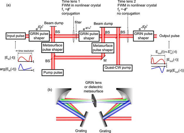
Figure 2. The proposed free-space temporal 4-f imaging system that time reverses and phase conjugates the input electric field in the time domain. (a) The schematic diagram of the free-space temporal 4-f imaging system. The quantity above each pulse shaper denotes the spectral phase the shaper induces. The first shaper can be adjusted to ensure that the pulse duration of the input pulse is greater than the time resolution of the system. The electric field envelope and the phase of a sample pulse are sketched for ideal spectral phase conjugation. See reference [32] for the experimental demonstration of a temporal 4-f imaging system. (b) The schematic diagram of the zero-dispersion GRIN (metasurface) pulse shaper. GRIN—gradient-index, BS—beam splitter, M—mirror.
Download figure:
Standard image High-resolution image3.3. Two-stage four-wave-mixing (FWM) process
The FWM process of the first time lens induces a second-order temporal phase to the input pulse. The field after the first time lens is

where  is the field after the first time lens,
  is the conjugate of the field before the first time lens, and Epump1(t) is the field of the chirped pump pulse for the first time lens with a perfect second-order spectral phase of exp(iϕ''ω2). This pump pulse must be synchronized with the input pulse, but both pulses need not originate from the same laser pulse. By adjusting the delay of the pump pulse, the frequency of the field after the first lens (
 ) can be tuned and isolated using a filter. The FWM process of the second time lens also induces a second-order temporal phase to the pulse. The field after the second time lens is

where  is the field after the second time lens, Elens2(t) is the field before the second time lens,
  with a perfect second-order spectral phase of exp(iϕ''ω2/2) is the conjugate of the field of the chirped pump pulse for the second time lens, and ECW(t) is the quasi-continuous-wave field. The frequency of the quasi-continuous-wave field is adjusted to generate an output with the same central frequency as the system input. According to the FWM processes (equations (7) and (8)), the CEP of the output pulse is CEPoutput = −CEPinput + CEPpump 1 − CEPCW. It is assumed that the pulse shapers are designed with 0 CEP. The continuous wave beam needs to be synchronized for a CEP with consistent value. If the pump pulse originates from the same laser pulse as the input pulse, then the first two terms become like terms and combine. If not, the pump needs to be CEP stable. The temporal 4-f imaging system does not require an intense pulse because the time lenses are based on FWM using pump lasers [32]. In fact, a weak input pulse is desired because high intensity can cause self-phase modulation.
4. Results
4.1. Temporal 4-f imaging system simulation
We simulated the processes involved in temporal 4-f imaging system using an input pulse with a central wavelength of λc = 1400 nm and a bandwidth of 0.05νc, where νc is the central frequency. The spectrum of this pulse supports the shortest-possible FWHM pulse duration of 34.6 fs, but this input pulse is chirped with ϕ'' = 4.4192 × 10⁻²⁷ rad−2 and a pulse duration of 701.4 fs. The coefficient of the second-order dispersion in this temporal 4-f imaging system is ϕ'' = 7.4430 × 10⁻²⁷ rad−2. The first pump pulse is time-shifted such that the second-order dispersion is centered around  νc. The output pulse of the temporal 4-f imaging system is plotted in time domain (figure 3(a)) and frequency domain (figure 3(b)). The spectral phase conjugation of the input pulse is plotted in time domain (figure 3(c)) and frequency domain (figure 3(d)). The spectrum measurement is accurate because it involves measuring a replica of the input pulse according to equations (1) and (5). The reconstructed pulse in time domain is plotted in figure 3(e) and it resembles the spectral phase conjugation (figure 3(c)). The spectral phase error of the output pulse compared to the spectral phase conjugation is plotted in figure 3(f). The range of the spectral phase error is 0.7% of the range of the spectral phase of the input pulse. The CEP of the simulated output pulse, however, is inconclusive because its value changes chaotically by changing the number of pixels used in the frequency axis, which has no impact on the real system. Another chirped input pulse with ϕ'' = 1.3258 × 10⁻²⁶ rad−2 and a pulse duration of 2100 fs undergoing an identical temporal 4-f imaging system is simulated. The output pulse is plotted in time domain (figure 3(g)) and frequency domain (figure 3(h)). The spectral phase conjugation of the input pulse is plotted in time domain (figure 3(i)) and frequency domain (figure 3(j)). The reconstructed pulse in time domain is plotted in figure 3(k) and it resembles the spectral phase conjugation (figure 3(i)) with very minor differences. The spectral phase error of the output pulse compared to the spectral phase conjugation is plotted in figure 3(l). The range of the spectral phase error is 1.1% of the range of the spectral phase of the input pulse. The increase in the error is due to the broadened input pulse while the temporal aperture, defined by the 1180 fs pulse duration of the second chirped pump pulse, stays the same. Due to this temporal aperture, the output pulse becomes significantly narrower in both time (figure 3(g)) and frequency domain (figure 3(h)) compared to the input pulse and the reconstructed pulse (figure 3(k)) with a 1.1% spectral phase error. If the input pulse broadens beyond the temporal aperture, the output pulse can give an entirely distorted result that does not represent the spectral phase conjugation. The temporal 4-f imaging system must then be readjusted by increasing ϕ'' of the temporal 4-f imaging system, which in turn increases the chirp of the pump pulses and the focal time of the temporal 4-f imaging system, for proper operation of the system.
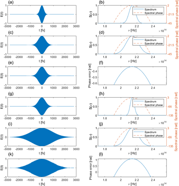
Figure 3. Simulated chirped Gaussian pulses undergoing the temporal 4-f imaging system with ϕ'' = 7.4430 × 10⁻²⁷ rad−2. The input pulses have a central wavelength of λc = 1400 nm and a bandwidth of 0.05νc. The input pulses are chirped with a pulse duration of (a)–(f) 701.4 fs, or (g)–(l) 2100 fs. (a) and (g) Time (b) and (h) frequency domain representation of the normalized electric field of the output pulse. (c) and (i) Time (d) and (j) frequency domain representation of the normalized electric field of the spectral phase conjugation of the input pulse. (e) and (k) Time domain representation of the normalized retrieved electric field of the PIE-PIE device. (f) and (l) Spectral phase error of the output pulse compared to the spectral phase conjugation.
Download figure:
Standard image High-resolution image4.2. Phase error reduction
Pulses with temporal features finer than the time resolution of a time lens will be distorted by the time lens, causing phase error in the spectral phase conjugation process. However, one can elongate the input pulse using the first pulse shaper in the temporal 4-f imaging system beyond the required dispersion to smooth out all temporal features and reduce the phase error. This is illustrated in figure 4 where pulses with the same third-order spectral phase where ϕ(3) = 3.9414 × 10−41 rad−3, but different second-order spectral phases are simulated. The input pulses have a central wavelength of λc = 1400 nm and a bandwidth of 0.05νc. The coefficient of the second-order dispersion in this temporal 4-f imaging system is ϕ'' = 7.4430 × 10⁻²⁷ rad−2. The input pulse with purely third-order spectral phase has temporal features as narrow as 20 fs (figure 4(c) is the spectral phase conjugation of the input pulse). The output pulse of the temporal 4-f imaging system (figure 4(a)) has spectral phase error with a range of 2.25 radian (figure 4(f)), which is 6.79% of the range of the input pulse's spectral phase (see figure 4(d)). This range is reduced to 0.48 radian as shown in figure 4(l) when the input pulse is broadened using a second-order spectral phase with ϕ'' = 6.6288 × 10⁻²⁷ rad−2 (figure 4(g) is the spectral phase conjugation of the input pulse). The reduction in phase error is because the input pulse has a significantly longer FWHM of 1090 fs without finer temporal features. The range of the spectral phase error as the coefficient of the second-order spectral phase ϕ'' varies is plotted in figure 4(m). The range of the spectral phase error first trends downward as ϕ'' increases up to 6.6288 × 10⁻²⁷ rad−2, followed by an uptrend. The final uptrend is due to the broadening of the input pulse beyond the 1180 fs temporal aperture as explained in the discussion of figure 3.

Figure 4. Simulated pulses with a cubic spectral phase where ϕ(3) = 3.9414 × 10−41 rad−3 undergoing the temporal 4-f imaging system. The input pulses have a central wavelength of λc = 1400 nm and a bandwidth of 0.05νc. (a)–(f) One of the input pulses is unchirped (g)–(l) while the other is chirped with (g)–(l) ϕ'' = 6.6288 × 10⁻²⁷ rad−2 (a) and (g) Time (b) and (h) frequency domain representation of the normalized electric field of the output pulse. (c) and (i) Time (d) and (j) frequency domain representation of the normalized electric field of the spectral phase conjugation of the input pulse. (e) and (k) Time domain representation of the normalized retrieved electric field of the PIE-PIE device. (f) and (l) Spectral phase error of the output pulse compared to the spectral phase conjugation. (m) Plot of the range of the phase error as the second-order spectral phase of the input pulse is varied. The encircled data point represents the two special cases that are shown.
Download figure:
Standard image High-resolution imageIn principle, our method can retrieve the unknown pulse regardless of the spectral phase error in the temporal 4-f imaging system because each output pulse corresponds to exactly one input pulse. The derivation of this one-to-one relationship requires robust simulations, and this will be explored in the future.
The temporal 4-f imaging system has a fundamental bandwidth limit of approximately an octave. This is because the spectrum of the pulse must be shifted by a positive amount beyond its bandwidth in the first time lens, isolated by a filter, and shifted back in the second time lens by adjusting the frequency of the quasi-CW pump laser [32]. If the full width of the spectrum of the input pulse is Δν, the frequency of the quasi-CW pump laser must be less than νc − Δν. This frequency should be greater than the UV frequency for the system to operate in free-space.
4.3. PIE-PIE simulations
The temporal 4-f imaging system simulations show that the system properly phase conjugates the input pulse with a few percent errors. For this reason, the simulations from now on assume an ideal temporal 4-f imaging system. We simulate a chirped pulse that has a Gaussian envelope with an FWHM of 58.9 fs and a central wavelength of 800 nm (figure 5(a)). The pulse has a linear instantaneous frequency that increases from 0.6νc to 1.4νc as time goes from −100 fs to 100 fs, and a non-zero CEP. A replica of the pulse is converted into vertical polarization, while the other replica with horizontal polarization is time-reversed and conjugated. The superposition of the two replicas in the time domain representing the output of the PIE-PIE interferometer is shown in figure 5(b). The two replicas are also converted into the frequency domain and superimposed at every wavelength as described by the Jones matrix equation (1). The polarization state at every wavelength is converted into Stokes parameters, which are plotted in figure 5(c). From the Stokes parameters, the spectral phase and spectrum are calculated using equations (4) and (5) respectively (see figure 5(d)). The transfer function of the phase conjugation process H(ω) is assumed to be 1. The calculated spectrum and spectral phase in figure 5(d) agree with the input pulse and accurately reconstruct it by equation (6 4). An unchirped pulse with a CEP of 0.3π, and all other parameters identical to the simulated pulse in figure 5(a) is simulated (figure 5(e)). The output of the PIE-PIE interferometer with equal arm lengths for this input unchirped pulse is simulated in the time domain (figure 5(f)). The Stokes parameters (figure 5(g)) representing the polarization state at every wavelength allow one to calculate the spectral phase and spectrum (figure 5(h)) directly using equations (4) and (5) respectively. The calculated spectrum and spectral phase accurately reconstruct the input pulse. It is important to note that an unchirped pulse has a constant spectral phase equal to its CEP. Therefore, the CEP of an unchirped pulse can be directly measured using only the measurements from a single wavelength. This CEP calculation only involves a matrix multiplication (equation (2)) to obtain the Stokes parameters and a straightforward formula to solve for the CEP (equation (4)). Therefore, the measurement of CEP of an unchirped pulse is only limited by the speed of the spectrometer, not the post-processing. Hence, the PIE-PIE device can be applied for CEP stabilization that requires rapid shot-to-shot determination of CEP at the repetition rate of the ultrafast laser.

Figure 5. Simulated chirped and unchirped pulse and their simulated outputs, along with the results of the PIE-PIE device's measurements. (a) Time domain representation of the normalized electric field real (E(t)) of a chirped pulse with a Gaussian envelope with an FWHM of 58.9 fs, a central wavelength of 800 nm, and an instantaneous frequency that increases linearly from 0.6νc to 1.4νc as time goes from −100 fs to 100 fs. (b) The simulated output of the PIE-PIE device with equal arm lengths using the simulated input of (a). (c) The Stokes parameters of the output pulse as a function of wavelength. (d) Normalized spectrum and spectral phase derived from the Stokes parameters using equations (4) and (5). (e) Time domain representation of the normalized electric field real (E(t)) of an unchirped pulse with a Gaussian envelope with an FWHM of 58.9 fs, and a central wavelength of 800 nm. (f) The simulated output of the PIE-PIE device using the simulated input of (e). (g) The Stokes parameters of the output pulse as a function of wavelength. (h) Normalized spectrum and spectral phase derived from the Stokes parameters using equations (4) and (5).
Download figure:
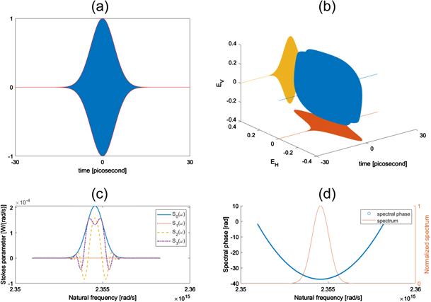
Standard image High-resolution imageOur technique is versatile and can be used for an arbitrary pulse duration at different wavelengths. To show that the PIE-PIE technique can be applied to long pulses, a chirped pulse with an FWHM of 9.42 ps is simulated in figure D1. Then, we simulate a heavily chirped Gaussian pulse, but with a different central wavelength of 400 nm (see figure 6(a)). The pulse has an FWHM of 58.9 fs. The instantaneous frequency increases linearly from 0.9νc to 1.1νc as time goes from −100 fs to 100 fs. The output of the PIE-PIE interferometer with equal arm lengths for this input pulse train is simulated in the time domain (figure 6(b)). The Stokes parameters (figure 6(c)) representing the polarization state at every wavelength allow one to calculate the spectral phase and spectrum (figure 6(d)) directly using equations (4) and (5) respectively. The calculated spectrum and spectral phase accurately reconstruct the input pulse.
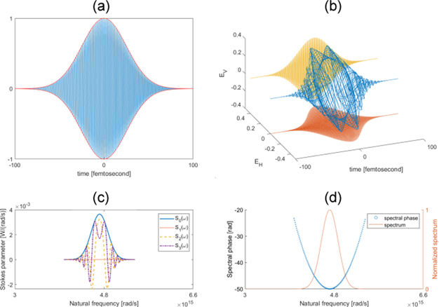
Figure 6. A simulated chirped pulse and its simulated output, along with the results of the PIE-PIE device's measurements. (a) Time domain representation of the normalized electric field real (E(t)) of a chirped pulse with a Gaussian envelope with an FWHM of 58.9 fs, a central wavelength of 400 nm, and an instantaneous frequency that increases linearly from 0.9νc to 1.1νc as time goes from −100 fs to 100 fs. (b) The simulated output of the PIE-PIE device with equal arm lengths using the simulated input of (a). (c) The Stokes parameters of the output pulse as a function of wavelength. (d) Normalized spectrum and spectral phase derived from the Stokes parameters using equations (4) and (5).
Download figure:
Standard image High-resolution imageNext, we simulate a pulse with complex shape and its simulated output after exiting the PIE-PIE interferometer. The Stokes parameters of this output at every wavelength is used to calculate the spectrum and spectral phase. The results of the simulation are shown in figure 7. The simulated pulse (see figure 7(a)) has an envelope that is a sum of two Gaussian functions. One is centered at t = 0 with an FWHM of 235.5 fs and the other is centered at 250 fs with an FWHM of 117.7 fs. The pulse has a linear instantaneous frequency that increases from 0.9νc to 1.1νc as time goes from −500 fs to 500 fs, and a non-zero CEP. A replica of the pulse is converted into vertical polarization, while the other replica with horizontal polarization is time-reversed and conjugated. The superposition of the two replicas in the time domain with a time delay of τ = 0 and τ = −120 fs are shown in figures 7(b) and (e) respectively. The two replicas are also converted into the frequency domain and superimposed at every wavelength as described by the Jones matrix equation (1). The polarization state at every wavelength is converted into Stokes parameters for the two cases, which are plotted in figures 7(c) and (f). From the Stokes parameters, the spectral phase and spectrum are calculated using equations (4) and (5) respectively (see figures 7(d) and (h)). The transfer function of the phase conjugation process H(ω) is assumed to be 1. We note that the second term in equation (5) representing the time delay is not critical in reconstructing the pulse as it simply shifts the reconstructed pulse in time. However, the time delay must be appropriately adjusted and kept small in the PIE-PIE device so the spectrally-resolved polarimeter can resolve the finest spectral fringe. Figure 7(g) shows the spectral phase without correcting for the 120 fs time delay. If the time delay is too large, it can cause phase jumps greater than π/4 in adjacent pixels and causes errors in the phase unwrapping of the spectral phase. The calculated spectrum and spectral phase in figure 7(h) agree with the input pulse and accurately reconstruct it by equation (6 4). Meanwhile, the calculated spectrum and spectral phase in figure 7(d) accurately reconstruct the negated version of the input pulse. This method has a possible sign error or equivalently an absolute phase error of π. This is because negating both the horizontal and vertical component of the polarization state in equation (1) yields the same polarization state.

Figure 7. A simulated pulse with complex shape and its simulated output, along with the results of the PIE-PIE device's measurements for two time-delay instances of τ = 0 and τ = −120 fs. (a) Time domain representation of the normalized electric field real (E(t)) of the simulated pulse. The envelope of the pulse is the sum of two Gaussian functions. One is centered at t = 0 with an FWHM of 235.5 fs and the other is centered at 250 fs with an FWHM of 117.7 fs. The instantaneous frequency increases linearly from 0.9νc to 1.1νc as time goes from −500 fs to 500 fs. (b) The simulated output of the PIE-PIE device using the simulated input of (a). (c) The Stokes parameters of the output pulse (b) as a function of wavelength. (d) Normalized spectrum and spectral phase derived from the Stokes parameters using equations (4) and (5). (e) The simulated output of the PIE-PIE device using the simulated input of (a) with the vertical polarization interferometer arm lengthened by 120 fs. (f) The Stokes parameters of the output pulse (e) as a function of wavelength. (g) and (h) Normalized spectrum and spectral phase difference derived from the Stokes parameters using equation (4) (g) before, (h) after correcting for the time delay term and equation (5).
Download figure:
Standard image High-resolution image5. Conclusion
In summary, we proposed the first technique through 'PIE-PIE' to directly measure the frequency domain electric field E(ω) with CEP information in a single-shot operation without any retrieval algorithm. The concept of PIE-PIE is to measure the spectral phase between the electric field and its phase conjugation, which can be realized by a time lens. As this phase conjugation process does not require the test pulse to be very intense, PIE-PIE can characterize an ultrashort pulse with relatively low intensity. This technique is real-time, only limited by the data acquisition rate of the spectrometer, allowing the PIE-PIE device to be applied for CEP stabilization that requires high-speed shot-to-shot determination of CEP. The ability to measure the spectrum, spectral phase, and CEP of low-intensity pulses will revolutionize the current field and enable studies of arbitrary non-repeating ultrafast events.
Acknowledgments
This work was supported by the Army Research Office and Bill & Melinda Gates Foundation.
Data availability statement
The data that support the findings of this study are available upon reasonable request from the authors.
Note
The authors declare no competing financial interest.
Appendix A.: Stokes vector
The Stokes vector is a vector that describes the polarization state of electromagnetic waves. The Stokes vector can be written as:

where the subscripts refer to the standard Cartesian basis ( ), and δ is the retardance. The retardance can be calculated by

where atan2(Y, X) returns the four-quadrant inverse tangent of Y and X.
Appendix B.: Spectral phase conjugation in frequency and time domain
Spectral phase conjugation is an operation on a pulse that inverts its phase in the frequency domain. This is equivalent to a time reversal and phase conjugation in the time domain. This relationship can be derived by Fourier transform as follows. First, we write the time domain electric field in terms of its Fourier transform

Conjugating both sides of the equation yields

To convert this equation in the form of a Fourier transform with the exponential of e−iωt , we substitute t with −t:

The above equation shows that a phase conjugation in the frequency domain is equivalent to a time reversal and phase conjugation in the time domain.
Appendix C.: Dispersion's effect on carrier-envelope phase (CEP)
In the following derivation, we show how the CEP of a pulse continuously changes as it travels through a dispersive medium. A single pulse can be written in the time domain as

Next, we substitute the term E(ω) in terms of its inverse Fourier transform  and equation (B2) becomes

Next, we group up the terms with the variable ω for the dω integral and define this integral as the propagator G(t − τ, z):

The wavenumber k(ω) can be Taylor expanded around the carrier frequency ωca into

The pulse in time domain (equation (B3)) becomes

If we substitute the time domain electric field in earlier time  where vg is the group velocity at the carrier frequency
  , we realize that it is related to the pulse of the present time with a phase change:

where vp is the phase velocity at the carrier frequency. The CEP is caused by the difference between the group and phase velocity of the dispersive medium as the pulse propagates through it. This can occur in a laser resonator due to intracavity dispersion and nonlinearities causing a slippage of the carrier-envelope offset from pulse to pulse. If the change in the CEO per resonator round trip is a constant (denoted Δφ), all optical line frequencies can be written as

where n is an integer index, νrep is the pulse repetition rate, and

is the CEO frequency that can be between 0 and νrep.
Appendix D.: Additional simulations
To show that the PIE-PIE technique can be applied to long pulses in the picosecond regime, we simulate a chirped Gaussian picosecond pulse with an FWHM of 9.42 ps in the time domain, a central wavelength of 800 nm, a linear instantaneous frequency, and a non-zero CEP (see figure D1(a)). The instantaneous frequency increases linearly from 0.999νc to 1.001νc as time goes from −30 ps to 30 ps. The output of the PIE-PIE interferometer with equal arm lengths for this input pulse train is simulated in the time domain (figure D1(b)). The Stokes parameters (figure D1(c)) representing the polarization state at every wavelength allow one to calculate the spectral phase and spectrum (figure D1(d)) directly using equations (4) and (5) respectively. The calculated spectrum and spectral phase accurately reconstruct the input pulse. Because the pulse duration of 9.42 ps is 2 orders of magnitude longer than that of the pulse in figure 5(a), the spectrum (figure D1(d)) of the picosecond pulse is significantly narrower than that of figure 5(d).
Figure D1. A simulated chirped picosecond pulse and its simulated output, along with the results of the PIE-PIE device's measurements. (a) Time domain representation of the normalized electric field real (E(t)) of a chirped pulse with a Gaussian envelope with an FWHM of 9.42 ps, a central wavelength of 800 nm, and an instantaneous frequency that increases linearly from 0.999νc to 1.001νc as time goes from −30 ps to 30 ps. (b) The simulated output of the PIE-PIE device with equal arm lengths using the simulated input of (a). (c) The Stokes parameters of the output pulse as a function of wavelength. (d) Normalized spectrum and spectral phase derived from the Stokes parameters using equations (4) and (5).
Download figure:
Standard image High-resolution image