


Abstract
When predicting complex systems one typically relies on differential equation which can often be incomplete, missing unknown influences or higher order effects. By augmenting the equations with artificial neural networks we can compensate these deficiencies. We show that this can be used to predict paradigmatic, high-dimensional chaotic partial differential equations even when only short and incomplete datasets are available. The forecast horizon for these high dimensional systems is about an order of magnitude larger than the length of the training data.

Original content from this work may be used under the terms of the Creative Commons Attribution 4.0 licence. Any further distribution of this work must maintain attribution to the author(s) and the title of the work, journal citation and DOI.
1. Introduction
For centuries, differential equation models derived from physical principles have been the preferred tool to forecast the behaviour of complex natural systems. More recently the advance of data-driven methods enabled many promising approaches for forecasting spatiotemporal system, e.g. with feed-forward neural networks [1], convolutional neural networks (CNN) [2] or reservoir computing [3]. In particular, chaotic systems are inherently difficult to forecast, as already the smallest deviations can lead to large errors later. Key challenges remain predicting complex systems that are high dimensional and chaotic, when only short time series and spatially incomplete data is available. We tackle these challenges by combining knowledge that we have about the governing equations of these systems with data-driven methods into a hybrid model.
We explore how hybrid methods help predicting complex, chaotic systems of which we only have incomplete and sparse knowledge. Every numerical, physical model of a natural system is incomplete in some sense, for example due to unknown parts of the dynamics, or due to deliberately omitting higher-order effects. Hybrid approaches try to account for these deficiencies with data-driven methods to derive more complete hybrid models.
The data-driven part of the hybrid models needs to be trained and when directly augmenting a differential equations with an ANN, it is no longer possible to use the standard backpropagation algorithm that is usually applied. Chen et al [4] presented an efficient algorithm to train through an ODE solver based on the adjoint sensitivity method. Rackauckas et al [5] expanded on this idea and developed the universal differential equations framework that allows to freely augment most types of differential equations with universal approximators such as ANNs. These approaches are also related to prior research that show how parameters of ODEs describing chaotic systems can be estimated, such as by Baake et al [6]. For the fully data-driven, and thus non-hybrid case, Sun et al [7] showed how the complete right-hand side of differential equations can be modelled with ANNs based on the neural ODE approach by Chen et al [4].
Another hybrid approach are physics-informed neural networks, which can approximate solutions of PDEs with ANNs and also set up ANNs whose outputs are solutions of a specific PDE [8]. Combining a knowledge-based differential equation model with a reservoir computer has also recently shown great promise for predicting chaotic systems like the Lorenz-63 and the Kuramoto–Sivashinksy (KS) equation [9, 10].
Combining knowledge of systems with data-driven approximations such as polynomials has been done for low-dimensional ODEs [[11], cf]. The approach that we aim for provides greater flexibility and capability through the use of ANNs as approximators and the possibility to use PDEs and their representations as high-dimensional ODEs through discretization.
In this article we focus on a particularly challenging situation: we want to predict the dynamics of high-dimensional chaotic systems by combining discretized PDEs with ANNs, under the condition of very short training datasets and with parts of the spatial data missing. The universal differential equations framework [5] provides the basis for the introduction of the neural partial differential equations (NPDE) that we will use. Compared to existing works, the results we are going to present in the following advance the field of hybrid modelling in two key aspects. First, we show that it is possible to train models based on very short training data, and second, we do that for chaotic systems even when the data is subjected to noise and incomplete.
We will first introduce the method of NPDEs and will then apply them to two prototypical, spatiotemporally chaotic systems: the complex Ginsburg Landau equation and the KS equation. We will show that our NPDE-based hybrid approach proposed here is capable of predicting the dynamics of these example systems in high spatial dimension and with only very short training data, compared to the forecast horizon.
2. Methods
The framework of universal differential equations [5] enables us to use universal approximators such as ANNs within partial differential equations (PDEs). The resulting NPDEs are hybrid models that are able to compensate missing parts of the PDE by learning them from data, thereby attenuating structural model errors. NPDEs are thus discretized PDEs with an ANN as part of the equation:

The ANN will mostly be comprised of densely connected layers of nodes Dense(x; Nin, Nout, fNL) = fNL(Wx + b), where the (Nout × Nin)-matrix W and the Nout-dimensional vector b are the trainable parameters Θi = {W, b} and fNL is a nonlinear function, here the swish function fNL(x) = x/(1 + exp(−x)) [12].

In order to train models like NPDEs, one needs to be able to compute gradients of the solution of differential equations with respect to the parameters of the equation, thus also of the ANN. Appropriate algorithms such as the adjoint sensitivity method were originally used, e.g., for sensitivity analysis of meteorological models [13]. Recent advances showed that these can also be used within the context of artificial neural networks [4]. In particular the universal differential equations framework made these methods much more accessible and easier to use [5]. The NPDE training and computations are all optimized to run on GPUs which enables us to investigate even very high dimensional systems efficiently.
The loss function that is minimized during the training process by a gradient descent algorithm is the sum of the least square errors of the predictions made by the NPDE and an additional parameter regularization of the ANN:

The sum is taken over all discretized spatial coordinates x and time steps it of the predicted trajectory. Throughout the article ||⋅||1 denotes the L1 norm and γ = 10−5.
In [5] non-chaotic applications of universal differential equations are discussed and these are usually trained by minimizing the mean square error of a relatively long trajectory predicted by the universal or neural differential equations. We found that it is to be difficult to train models for chaotic processes on long trajectories as inherently small deviations at the start of the trajectory can lead to massive deviations later. We thus integrate the NPDE only from t0 to t0 + iτ Δt for a small iτ and repeat this from every initial condition in the training dataset. For iτ = 1 we therefore train on the one-step-ahead forecast error. Increasing the length of the integration interval also increases the computational complexity massively. We thus first integrate with iτ = 1 until the forecast error on a validation set converges and then slowly increase iτ to its final value τ. The final length of the integration interval τ is a hyperparameter of the training procedure. When integrating the NPDE, we save the trajectories at constant sampling time steps Δt for better comparability, even though the solvers will typically feature adaptive step size control. Depending on the model in question, Δt might need to be quite small to ensure a successful training, as we will address later.
In order to model possible derivatives in the unknown parts of the PDE, we introduce a novel trainable layer, the Nabla layer ∇. It is defined by

where ∇FD is the finite difference derivative matrix and w is a trainable parameter. The second term of the right-hand side is thus a scaled, numerical first derivative of the input, and the layer learns whether or not to take a derivative of the input (or a linear combination of both input and its derivative). The parameter w is approximately bound to the interval [−1; 1] by an additional penalty in the overall loss function. For this function we chose p(w) = max(x6 − 1, −x4 + x2) because it has large values outside of [−1; 1] and local minima at 0 and ±1. When stacking k of these layers and a multi-layer perceptron (MLP) together, we are able to model functions of derivatives up to order k. To increase the numerical precision of the Nabla layer, we use alternating forward and backward finite difference schemes when stacking Nabla layers as we noticed an impact of the accuracy of the finite difference schemes on the results, especially when higher order derivatives are modelled. While we investigate only a finite difference scheme here, using other discretization approaches are likely to work as well and could be investigated in future research. Additional skip connections can help training these models if they are comprised of many layers, resulting in a residual network (ResNet) [14].
Since we directly augment the differential equation, the NPDE approach is very flexible. It does not have a fixed input or output dimension. We could integrate the trained model in higher or lower resolutions, or as we deal with systems where local interaction are dominant, the NPDE approach enables us to deal with spatially incomplete data as well. We can learn the missing part of the equations from the incomplete data and predict the complete systems by defining a 'learn domain' that is situated well within the known data (see figure 1). The initial conditions for each integration are 0 where we have no data and the loss function is computed only from points within this learn domain. In these cases we only integrate for one sampling time step and are thus using a one-step-ahead error, as longer integration intervals would allow the propagation of features outside of the known domain to the inside of the learn domain.

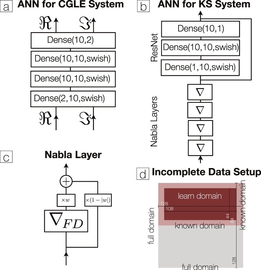
Figure 1. Overview of learning setups. (a) ANN setup for the CGLE system. and are the real and imaginary part of the value of u(x, t) u(x, t). (b) The ANN setup for the KS system comprises four Nabla layers and a ResNet. (c) Nabla layers used in (b), the parameter w is trainable. ∇FD is the finite difference derivative matrix. (d) Sketch outlining the setup to learn the NPDE from spatially incomplete data.


Download figure:
Standard image High-resolution image3. Results
In the following we will assume that we know only a part of the equation we are investigating and 'forget' about another part of the equation, which is instead modelled by an artificial neural network . The latter part will be trained with data. For this theoretical setup, we generate this data from the true, known system and then compare it with the prediction of the trained NPDE.

We assess how well the NPDEs perform by first integrating them from the first initial conditions that were not part of the training part for a suitably long time. Importantly, when integrating we save the trajectory at the same regular sampling time steps Δt as when generating the initial true data. We then define the following measures of forecast accuracy: the non-normalized error

and the normalized error [9]

where ||⋅||2 is the L2 norm. As defined in [9], we also compute a valid time tv as the first time when e(tv) > 0.4. The time will be either expressed in the number of forecasted sampling time steps Nf, or by scaling it with the maximum Lyapunov exponent as a natural time scale of the system.
The results of our NPDE approach will be compared to other methods. The first benchmark is a CNN with a bottleneck, similar to [15]. Another comparison is a hybrid reservoir computer [9] that also combines a knowledge-based model with a data-driven model, i.e., the incomplete PDE with a reservoir computer. For high-dimensional systems, the size of the reservoir network needs to be increased accordingly. For the systems investigated here, the necessary reservoir size becomes potentially prohibitory large. For our comparative purposes, we thus compute the hybrid reservoir with a lower-dimensional system with the same inter-grid spacing. Additionally, we also show how the incomplete model on its own performs as a predictor. Further details on these comparisons can be found in the appendices
3.1. Complex Ginsburg–Landau equation
The complex Ginsburg–Landau equation [16, 17] is defined by

where u(x, t) is a complex valued field on two spatial dimensions. The CGLE is a prototypical equation that models every reaction-diffusion system close to the onset of oscillation [17]. For various parameter configuration, like α = 2, β = −1 as chosen here, this system exhibits chaotic behaviour. The physical size of the domain is set to 192 × 192 in arbitrary physical units and periodic boundary conditions are applied. The domain is then discretized with a finite difference scheme to a grid with 128 × 128 nodes, thus transforming the PDE into a 16 384-dimensional ODE. Here, we focus on modelling the reaction term with an ANN. The NPDE we investigate here is given by

As part of the NPDE is defined in a way that it only has as a single input: the value of the spatiotemporal field u at one specific position. Since u is complex valued, the real and imaginary part are split as separate inputs. is a multilayer perceptron with two hidden layers, each with 10 densely connected nodes (see figure 1).


A single long trajectory of the CGLE is integrated with a Tsitouras solver [18]. The initial conditions are uniformly random within the interval [−0.005; 0.005] for both the real and imaginary part. Although the solver has an adaptive step size, the trajectory is saved every Δt = 0.1. The first 2000 steps are not saved to avoid any transient dynamics. Only the next 25 steps after the transient are the training set and the remainder of the trajectory is saved for validation and test set. The NPDE is trained minimizing the loss function equation (2) using a stochastic gradient descent with weight decay [19].
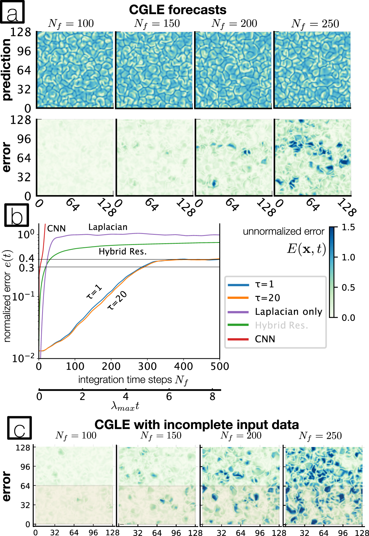
Figure 2 shows the prediction of the trained NPDE for different time steps Nf and how the normalized error evolves. We found that the NPDE makes accurate predictions that exceed the length of the training set by far. The normalized error increases exponentially with increasing t until it levels off at around 0.4, which coincides with the threshold of the valid time tv for the CGLE NPDE. Therefore, we additionally measure when e(t) = 0.3 is reached for the first time.

Figure 2. NPDE forecast for the CLGE. (a) Shows the prediction made by the NPDE for four different time steps Nf and the difference of this prediction to the true value. We show the absolute value of these fields here. (b) Is the evolution of the normalized error e(t) for two different integration lengths and compared to a hybrid reservoir, a CNN and the forecast made by integrating the Laplacian only. The upper x axis is given in units of integration time steps with Δt = 0.1 and the lower axis is in units of the Lyapunov time. (c) Shows the CGLE forecast with incomplete input data from only the shaded area at the bottom of the spatial field.
Download figure:
Standard image High-resolution imageThe valid time increases slightly when the final length of the integration interval τ is increased (see figure 2), however increasing τ needs considerably more computation time. Ultimately, this increase is so small that it does not seem to justify the much higher computation time in the case of the CGLE. The valid time is Nf = 388 sampling time steps, for τ = 1 and Nf = 479 for τ = 20, whereas e(t) = 0.3 is reached for Nf = 286 for τ = 1 and Nf = 292 for τ = 20. Given a maximum Lyapunov exponent of λmax ≈ 0.167 and Δt = 0.1, this is equivalent to 4.88λmax t to reach e(t) = 0.3 and a valid time of 8.01λmax t for τ = 20. In comparison, the valid time of the hybrid reservoir is Nf = 25 or 0.44λmax t. For the CNN it is Nf = 8 or 0.13λmax t.
Additionally, we investigated the sensitivity of the NPDE approach to noise in the underlying data by adding a small, normally distributed noise vector to the part of the trajectory x(t) that was used for training. We use only one constant noise vector

where each element of η(t) is independently drawn from a normal distribution . In this way we simulate observational noise. For a given standard deviation of the noise, we train the model in the same manner as before, with 25 time steps of training data xη . The forecast error e(t) can be evaluated by comparing the NPDE forecast against the original time series x, or against the series with noise xη . In our trials the forecast length did not differ significant from each other in either case. In figure 3 we report the results for noise with a standard deviation between 0.01 and 0.2. One can see a relatively smooth response to the increased observational noise. The forecast length decreases, but even at σ = 0.2 meaningful forecasts can still be made. In the appendix table 1, forecast times are reported for the various noise levels.


Figure 3. Normalized forecast error according to equation (5). The coloured numbers indicate the standard deviation of the noise used for the trial with the normalized error in the same colour. The CGLE has a mean standard deviation (in time) of σ ≈ 1.3.
Download figure:
Standard image High-resolution imageAccurate forecasts can even be made with incomplete data as results presented in figure 2 show when only one half of the spatial field was used to train the NPDE. The valid time is Nf = 333 sampling time steps or 5.57λmax t. The slightly lower threshold e(t) = 0.3 is reached at Nf = 254 sampling time steps or 4.24λmax t. There is no significant difference between the accuracy inside and outside of the known domain as the almost identical evolution of the normalized error shows.
3.2. Kuramoto–Sivashinsky equation
Another paradigmatic example of a spatiotemporally chaotic PDE is the KS equation

This equation is solved again with a finite difference scheme and periodic boundary conditions and length L = 1160. We discretize it to 4096 spatial grid points and solve for a long trajectory of which we use a Nt = 25 long training dataset at Δt = 0.02 sampling time steps. For the NPDE approach we 'forget' the term with the second derivative and replace it with an ANN consisting of four Nabla layers and an MLP with a residual connection (see figure 1), so that the NPDE reads

During the training procedure the parameters of the Nabla layers that we introduced in equation (3) quickly converge to two being very close to 0 and two very close to 1, thus correctly identifying the order of the derivative that is missing in the incomplete model. Figure 4 shows the results of the predictions of the NPDE. The valid time tv is 2891 time steps which, given a maximum Lyapunov exponents λmax = 0.07, is equivalent to 4.05λmax t. The normalized error increases exponentially with increasing t. The hybrid reservoir can predict accurately up to a valid time of Nf = 52 or 0.08λmax t.

Figure 4. NPDE forecasts for the Kuramoto–Sivashinsky equation. Predictions of the NPDE in the top row and difference to the true values in the bottom row. The right-hand-side panels show a detailed view of the area marked in pink in the large plots on the left. The valid time tv is marked in the difference plots.
Download figure:
Standard image High-resolution imageWe found that especially for the KS system, the forecast profits from smaller values for the sampling time step Δt. This became most apparent when tasking the NPDE model with replacing the forth derivative term, as is shown in the appendix
4. Discussion
Using NPDE one is able to make forecasts of only partially known high-dimensional chaotic systems, even when datasets available for training are extremely short and spatially incomplete. Importantly, we showed that our NPDE approach works best for chaotic systems with short integration intervals and small sampling time steps. Due to the chaotic nature of the investigated systems, training has to start by integrating only a single sample time step ahead, before slowly increasing the integration interval. However, for the prototypical systems that we investigated here, longer integration intervals do not significantly improve forecasts made by the NPDE. This should change when non-Markovian systems are investigated. Additionally, we introduced a novel finite-difference layer that enables the NPDE approach to work well with systems such as the KS system, as well when e.g. diffusive effects are modelled.
Essentially, the NPDE approach makes use of the ergodicity of such systems and is thus able to train and make accurate forecast not despite but because these systems are high dimensional. In the setups we used the ANNs are an efficient tool due the uniformity of the domain and their capability to fit any right-hand side of the equation as long as enough training data is available. Despite the short time series, the large amount of spatial information give us enough data to train the artificial neural networks, even when the training data is subject to observational noise. The forecast horizon of the NPDE is much longer than the dataset used for training itself and as the differential equation is modelled directly, one can also make predictions from arbitrary initial conditions. In many fields such as climate science often datasets are rather short, so that the capability to be trained on such short datasets could prove extremely valuable. The CGLE system we investigated is 16 384-dimensional, whereas the KS system is 4096 dimensional. The NPDEs are optimized on GPUs and thus the approach is scalable and increasing the dimension further is certainly possible. The key challenges that we identified: high-dimensionality, chaotic behaviour, short time series and incomplete data are all successfully tackled by using NPDEs. As we showed, NPDEs are also useful in cases where only incomplete data is available. While this approach seems to be limited to systems without significant long-range interactions, it is still a powerful tool that enables predictions even when not the complete spatial domain is available as training data.
Based on these results we conclude that NPDEs are a promising approach with a wide range of possible applications, especially because they solve one of the crucial limitations of machine learning: the need for long training datasets. In the future we hope to apply this method to experimental data from nonlinear optics on the one hand, and from atmospheric dynamics, on the other hand. General circulation models of the atmosphere seem to be an ideal application for our NPDE framework. Although very sophisticated models exist, they cannot resolve every possible influence and scale, which traditionally leads to parameterizations of the unresolved scales and processes such as cloud formation. In addition, the length of available observational training data is relatively short compared to the time scales of many phenomena in climate dynamics or in physiology, economy and ecology.
Data availability statement
All data that support the findings of this study are included within the article (and any supplementary files).
Acknowledgments
This paper was developed within the scope of the IRTG 1740/TRP 2015/50122-0, funded by the DFG/FAPESP. The authors thank the German Federal Ministry of Education and Research and the Land Brandenburg for supporting this project by providing resources on the high performance computer system at the Potsdam Institute for Climate Impact Research. NB acknowledges funding by the Volkswagen foundation and the European Union's Horizon 2020 research and innovation programme under Grant agreement Nos. 820970. JK acknowledges funding by the Russian Ministry of Science and Education Agreement No. 13.1902.21.0026. We wish to acknowledge the authors of the Julia libraries DiffEqFlux.jl [5], DifferentialEquations.jl [20] and Flux.jl [21] that were used for this study. Especially, we like to thank Christopher Rackauckas for his work on DiffEqFlux.jl and DifferentialEquations.jl and any help when problems with the libraries arised.
Appendix A.: Kuramoto–Sivashinsky model—4th-order derivative term
In the main text of this article, when investigating the KS equation, we replaced the second order term with an ANN. Here we show additional results to demonstrate the robustness of this approach. For this purpose we replace the term with the forth-order derivative with an ANN:

When investigating this setup, it became even more apparent that small values for the integration time step Δt are needed. Whereas the training fails for Δt = 0.1, the results shown in figure 5 for Δt = 0.02 are similar to those reported in the main text for the second derivative term. The valid time tv is 2953 time steps which, given a maximum Lyapunov exponent λmax = 0.08, is equivalent to 4.72λmax t.

Figure 5. Results for the NPDE for the KS system according to equation (A1). The right-hand panels show a zoomed in view of the area marked with the magenta rectangles in the left-hand panels.
Download figure:
Standard image High-resolution image
Table 1. Results for observational noise with the CGLE setup: integration time step at which the normalized error e(t) first passes 0.3 and 0.2 for various values of observational noise σ.
| σ | 0.01 | 0.02 | 0.04 | 0.06 | 0.08 | 0.1 | 0.12 | 0.14 | 0.16 | 0.18 | 0.2 |
|---|---|---|---|---|---|---|---|---|---|---|---|
| t0.3 | 259 | 209 | 147 | 125 | 106 | 97 | 95 | 92 | 90 | 88 | 89 |
| t0.2 | 207 | 161 | 106 | 83 | 69 | 59 | 54 | 46 | 40 | 35 | 30 |
Appendix B.: Hyperparameter choice
In our article we made several hyperparameter choices that we are going to explain in the following. First of all, we experimented with the numbers of ANN nodes, between 10 and 30, and noticed little difference in the results, so that we chose the smaller amount of nodes. The regularization has little to no influence on the results for the CGLE and was only used there for consistency with the approach that we used for the KS model. For the KS model, introducing a regularization did improve the results. However, the regularization is still quite small compared to the initial least-squared error of the spatiotemporal field, as we are working with such a high-dimensional field. In terms of the activation function we tested ReLu, SeLu and Swish and found Swish to be working best.
Appendix C.: Convolutional neural network
The results of the NPDE forecast are compared to corresponding ones obtained with a CNN. This CNN is set up with a bottleneck, meaning that the first convolutional and pooling layers reduce the dimension of the input before subsequent layers extend the dimension back to the full size of the field. It makes forecasts by using a recursive loop in which the output of the CNN is fed back as input for the next time step. This architecture showed to be successful in approximating complex spatiotemporal fields, like simple global circulation models [15]. The CNN consists of three convolutional layers with 3 × 3-sized kernel, each with 8 channels and each followed by a 2 × 2 max pooling layer. The dimension is reduced, this is the so-called 'bottleneck' of the CNN. Then, three convolutional layers with 3 × 3-sized kernel, each followed by an upsampling layer, scale the dimension back to the input dimension. The CNN is trained by minimizing the one-step-ahead least-squared forecast error with a stochastic gradient descent method over 10 000 epochs of the dataset. The exact setup that we investigate is one where CNNs cannot excel easily. The reason the CNN approach is leading to worse results than the neural PDE is the very short training data combined with the high dimensionality of the training data. It would likely perform much better with training datasets of lengths of a few thousand samples. Nevertheless, the comparison we present highlights the strength of our hybrid NPDE approach in exploiting the spatial structure to allow to be trained on very short time series.
Appendix D.: Hybrid reservoir
Combining knowledge-based but incomplete models with a data-driven numerical model has previously been achieved successfully using reservoir computers. Pathak et al [9] showed that such a setup is able to forecast chaotic processes for very long times. However, in these examples very long input datasets were used. Here, we use the same basic setup as reported in [9] with reservoir size N = 20 000, spectral density ρ = 0.4, sparsity ⟨d⟩ = 0.03, input coefficient uniformly drawn from [−0.5; 0.5] and regularization constant 10−4. The knowledge-based model is the NPDE without the neural network, thus the PDE with one term missing. It was integrated using the LSODA solver from the Fortran ODEPACK library. While for longer training datasets a forecast horizon of several Lyapunov times can be achieved, it is much lower for the short training datasets explored in this article. For the 128 × 128-sized grid that is used for the CGLE and the 4096-dimensional KS discretization, one would need much larger reservoir sizes. These are potentially prohibitively large. We therefore computed the hybrid reservoir comparisons on smaller grids, 50 × 50 for the CGLE and 128 for the KS.
Appendix E.: Source code
The source code is available at https://github.com/maximilian-gelbrecht/NPDEChaos/.