


Abstract
Collective dynamics in lithographically-defined artificial spin ices offer profound insights into emergent correlations and phase transitions of geometrically-frustrated Ising spin systems. Their temporal and spatial evolution are often simulated using kinetic Monte Carlo (kMC) simulations, which rely on the precise knowledge of the switching barriers to obtain predictive results in agreement with experimental observations. In many cases, however, the barriers are derived from simplified assumptions only, and do not take into account the full physical picture of nanomagnetic switching. Here we describe how the immediate magnetic square- or kagome-ice environment of a nanomagnet reversing via quasi-coherent rotation can induce clockwise and counter-clockwise switching channels with different barrier energies. This energy splitting for chiral reversal channels can be sizeable and, as string-method micromagnetic simulations show, is relevant for artificial spin ice systems made of both exchange- as well as magnetostatically-dominated units. Due to the barrier splitting and further reductions due to non-uniform reversal, transition rates can be exponentially enhanced by several orders of magnitude compared to mean-field predictions, especially in the limit of rare switching events where thermal excitation is less likely. This leads to significantly faster relaxation time scales and modified spatial correlations. Our findings are thus of integral importance to achieve realistic kMC simulations of emergent correlations in artificial spin systems, magnonic crystals, or the evolution of nanomagnetic logic circuits.
Export citation and abstract BibTeX RIS

Original content from this work may be used under the terms of the Creative Commons Attribution 4.0 licence. Any further distribution of this work must maintain attribution to the author(s) and the title of the work, journal citation and DOI.
Artificial spin ice systems are lithographically-created lattices of elongated single-domain nanomagnets, and have been designed to investigate the effect of correlations and the onset of long-range order in frustrated two-dimensional magnetic lattices [1–4]. Of particular interests is the evolution of extended spin ice lattices from a field-saturated state towards an energetically favourable (ground) state, driven by thermally-activated reversal of individual nanomagnets. Such experiments have been performed mainly using photoelectron emission microscopy, and gave valuable insight on the relaxation process and the formation of spatial correlations [5–9].
The understanding of experimentally-observed temporal evolution of extended spin ices are often guided and supported by model predictions, for example from kinetic Monte Carlo (kMC) simulations. Their major advantage over full micromagnetic simulations is that they are less computational costly, and thus can be extended to larger systems and longer time scales. This coarse-grained approach, which disregards microscopic details of the moment reversal, allows to simulate systems with a large number of moments evolving over long time scales, which otherwise would be too computationally-costly to be implemented in full micromagnetic simulations.
To obtain correct relaxation time scales and spatial correlations, kMC simulations rely instead on the precise knowledge of the rates for individual moment reversal. To match the measured experimental time scales the two main parameters determining the switching barriers used in the kMC simulations—the single-particle barrier and the interaction strength—are often adjusted [7, 9–11]. These changes, however, are usually derived from simplified or approximative assumptions only or associated with extrinsic influences, which do not take into account the full physical picture of nanomagnetic switching. Furthermore, an often-used mean-field approach does not consider the intrinsic freedom for clockwise or counter-clockwise rotations [7, 8, 12–14], which can lead to distinct switching barriers, as we previously showed [15].
In this work, we derive that a net perpendicular field from a defect-free double-vertex environment acting on the switching nanomagnet enables favourable chiral reversal pathways in artificial square and kagome ice. Using artificial square ice as an instructive example, we compare switching barriers obtained from micromagnetic string-method simulations for exchange- and magnetostatic-dominated geometries to those derived from simplified point-dipole predictions. We find that the latter consistently overestimates the barriers and underestimates the chiral splitting of the former, and are not applicable even with renormalised parameters in the case where non-coherent reversal modes are possible.
Reductions and splitting of the switching barriers lead to exponentially enhanced transition rates especially in the limit of rare events, as we show with a modified Arrhenius law. Using the rates for the chiral transition channels as input for kMC simulations, we find that the evolution of an extended square ice proceeds much faster, and involves different spatial correlations when compared to a mean-field model.
The influence of the immediate environment on the nanomagnetic switching thus is a key ingredient to correctly model the relaxation dynamics of artificial spin ices, as well as of functional magnonic materials and small-scale circuits for computation. We therefore expect our results to be relevant to different communities making use of thermally-driven relaxation of interacting nanomagnets.
This work is structured into three sections: in section 1 a basic understanding is derived on how the magnetic environment can lead to chiral switching channels in artificial square ice. Section 2 compares point-dipole model predictions to micromagnetic simulations of nanomagnets of different dimensions and material parameters. In section 3, ramifications of the modified switching barriers on the switching rates of single nanomagnets and relaxation kinetics of extended artificial square ice are discussed.
1. Chiral moment reversal
Artificial spin ices are lithographically-designed magnetic metamaterials with identical nanomagnets arranged on lattices with different geometries [1–4]. In the following, we focus our discussion on the example of artificial square ice, in which nanomagnets are arranged on a square lattice with periodicity a, see figure 1(a).

Figure 1. Switching barriers in artificial square ice. (a) Nanomagnets are arranged on a square lattice with periodicity a. The strongest mutual interaction JNN acts between perpendicular nearest-neighbour moments mj
. (b) Fully-magnetised double-vertex state #0, with enumeration of moments. The central nanomagnet (black) can rotate either clockwise (red arrow) or counter-clockwise (blue arrow) from left (←) to right (→). (c) Energetically-favourable states, on the left, feature more head-to-tail configurations between the central and neighbouring moments (green arrows). (d) In a perturbative picture, the switching barrier energies can be obtained by adding the interaction energies to the switching barrier ΔEsb of an isolated nanomagnet. If only the energies of the equilibrium configurations (←, →) are taken into account, a mean-field barrier is obtained (gray arrow to cross). In case the environment features a perpendicular magnetisation, i.e.  , the high-energy states (↑, ↓) will split, and thus yields separate transition barriers for clockwise (red) and counter-clockwise (blue) rotation.
Download figure:
Standard image High-resolution imageDue to their shape anisotropy, each stadium-shaped nanomagnet with length l, width w, and thickness t is quasi-uniformly magnetised, and thus behaves like an Ising macrospin. Without applied field or interactions with neighbours, the magnetic moment will align with the long axis, i.e. to the left (←) or right (→) if considering the black nanomagnet in figure 1(a). To spontaneous switch between these energetically-degenerate configurations (without loss of generality from ← to →), the moment rotates to overcome a metastable state for which the net moment points along the nanomagnets' short axis, i.e. ↑ or ↓. The difference between the metastable and equilibrium micromagnetic energies Emm gives the single-nanomagnet switching barrier ΔEsb:

The value of ΔEsb depends on the size, shape and material of the individual elements [16–19]. For the assumption of uniform magnetisation, the barrier is given by the shape anisotropy  , with V being the volume of the nanomagnet. Values of Kshape are either tabulated for ellipsoidal geometries [20] or can be calculated via magnetostatic simulations [21, 22].
The mutual coupling between nanomagnets is given by magnetostatic interactions, which takes the following form between point-dipole moments mi and mj separated by a distance vector rij = ri − rj :

In artificial square ice the strongest coupling, denoted by JNN, occurs between nearest-neighbour nanomagnets at a 90° angle, see figure 1(a). Using the lattice periodicity a and the net moment m = |m| = Msat
V of a nanomagnet with volume V and material saturation magnetisation Msat, we define a convenient energy scale  :
:

Due to the pronounced distance dependence, Edip ∝ r−3, the coupling between nanomagnets meeting at the vertex points highlighted in figure 1(a), is dominant over further-range interactions [23, 24]. Therefore, we investigate the switching barriers for moment reversal of a central nanomagnet under the influence of its closest neighbours only.
1.1. Switching environments
For an infinite artificial square ice the environment that influences the reversal of a nanomagnet forms a double-vertex configuration, as depicted in figure 1(b). Here, each tip of the central nanomagnet (black) is in close interaction to three other nanomagnet (gray), whose magnetisation remains largely unchanged during the reversal of the central nanomagnet. The extended square lattice then can be considered as an infinite tiling of these motifs.
We denote each magnetic equilibrium configuration with a state number #i determined by the arrangement of the surrounding nanomagnets, and the orientation of the central (switching) nanomagnet, which can point to the left (←) or to the right (→). The state number #i can be obtained from the binary representation of the relative configuration of the six surrounding nanomagnet numbered 1 to 6 according to the scheme shown in figure 1(b):

Half of the 26 = 64 environment configurations of the double vertex are depicted in figure 2. The remaining states #i can be derived by applying a time reversal operation on the configurations #(26 − 1 − i).

Figure 2. Enumeration of double-vertex states. (a) Based on the dipolar energies  of the environment configurations #i where the central moment can point in different directions, k = ←, →, ↑, ↓, five classes can be distinguished (highlighted with different colours). Configurations with a magnetisation
  perpendicular to the central nanomagnet feature distinct barriers for nanomagnet reversal via clockwise and counter-clockwise rotation. (b) Environment configurations #0 to #31 sorted into the five categories. In total, 40 out of the 64 environment states promote switching with a favoured chirality.
Download figure:
Standard image High-resolution image1.2. Switching barriers from a point-dipole model
In the following, we discuss a perturbative approach to switching barriers in artificial square ice. Here, the single-nanomagnet barrier ΔEsb, figure 1(d), is modified due to energy contributions arising from the interactions with the immediate magnetic environment.
To discuss a specific example, we focus on the fully-magnetised double-vertex environment #0 depicted in figure 1(b). The energy of the configuration where the central moment points (exactly) to the left, ←, is lower than when it points to the right, →, where three magnetic charges meet at each vertex point. Using simplified assumptions and symmetry arguments, one can derive a mean-field switching barrier  (as the average of the barriers for clockwise and counter-clockwise rotation, see appendix

This mean-field barrier, however, is missing a crucial point, as independent relaxation pathways via clockwise and counter-clockwise rotation of the central nanomagnet need to be considered, i.e.

and

These barriers are not necessarily equivalent, as shown in figure 1(c): due to their staggered spatial arrangement, the central moment in a fully magnetised environment #0 will preferably align ferromagnetically with its neighbours, thus forming a head-to-tail flux-closure configuration which reduces the dipolar energy term in equation (2). Therefore, transitions via counter-clockwise rotations (blue) of the central nanomagnet will be largely favoured over those via clockwise rotations (red).
From the dipolar energies for all environmental states and orientation of the central moment, figure 3(a), one can obtain the respective clockwise and counter-clockwise switching barriers, figure 3(b). Under the assumption that ↑ and ↓ align perfectly along the short axis of the nanomagnets, the energy splitting between the configurations is symmetric around the mean-field barrier  (marked by crosses), and equals the three distinct values shown in figure 3(c).

Figure 3. Barrier splitting in a double-vertex environment, based on the point-dipole model for moment reversal. (a) Normalised dipolar configuration energies  of a central moment k pointing to the left k = ←, top k = ↑, right k = →, or bottom k = ↓ (as indicated with triangles) embedded in environments #i (labelled on the top). The colour code corresponds to the scheme presented in figure 2. (b) Chiral switching barriers
  and
and  are marked by large and small circles, respectively, and the mean-field barrier by a cross. (c) For environments with finite perpendicular magnetisation
  acting on the central nanomagnet a splitting between clockwise and counter-clockwise barriers is observed (marked in yellow, red and blue). The energy splitting predicted by equation (9), and normalised to
  , is marked by dashed lines.
Download figure:
Standard image High-resolution imageBarrier splitting occurs for all environments which feature a perpendicular effective field  generated by the neighbouring nanomagnets, that acts on the central nanomagnet (indices bj
are as defined in equation (4)):
generated by the neighbouring nanomagnets, that acts on the central nanomagnet (indices bj
are as defined in equation (4)):

The normalised perpendicular magnetisation  can take the values of 0 (black and purple in figures 2 and 3), ±2 (orange), and ±4 (red and blue) only. Thus, we can modify equation (5) to include an additional energy term:

For a central moment initially pointing to the left (←), the second term (derived in appendix
In conclusion, with a simplified point-dipole model the switching barriers are modified by the choice of clockwise vs counter-clockwise rotation, if the moment interacts with an effective perpendicular stray field generated by its environment. As shown in figure 2, 40 out of the 64 double-vertex configurations of artificial square ice feature a finite perpendicular magnetisation  acting on the central nanomagnet. In particular, we expect a maximum chiral barrier splitting for the fully-magnetised environments (marked in red), which are commonly-used initial states for thermal relaxation studies of artificial spin ice [7].
The conclusions of this section are of general validity for arrays of interacting nanomagnets. The calculation of switching barriers for clockwise and counter-clockwise transitions can be easily adapted to other moment configurations. As an example, in supplementary material (https://stacks.iop.org/NJP/23/033024/mmedia) figure 1 we show that chiral barrier splitting occurs in over 60% of the moment configurations of artificial kagome spin as well.
The existence of separate chiral switching channels is by no means a curiosity, since nanomagnetic switching will occur predominantly via the more favourable pathway. We thus expect profound consequences on the switching rates and transition kinetics when taking into account the chiral splitting.
2. Micromagnetic switching
The point-dipole switching barriers represent a perturbative approach parametrised by two parameters only: first, ΔEsb describes the switching barrier of an isolated nanomagnet, and implicitly depends on its shape and size [20]. Second,  quantifies the energies of equilibrium configurations due to the interactions between nanomagnets placed on the square lattice, and modify the switching barrier of individual nanomagnets. The mean-field energy barrier in equation (9), however, does not take into account possible non-coherent moment reversal. In particular, it does not describe the influence of material parameters such as the saturation magnetisation Msat and the exchange strength Aex, thermal fluctuations, and the magnetic environment. Due to these effects the net moment can be dynamically reduced during reversal, e.g. via non-uniform buckling modes, vortex creation, or domain formation [25–28].
To have a nuanced look on how the energy barrier depends on (1) the material parameters, (2) the nanomagnet shape and size, and (3) the interactions with neighbouring nanomagnets, we now turn to a full micromagnetic simulation of the reversal barriers.
2.1. Implementation of string-method simulations
Contrary to simulations employing the Landau–Lifschitz–Gilbert equations to explicitly solve the time-dependent evolution of the nanomagnetic reversal, we determined the associated energy barrier using a time-independent string method. In this approach, starting from a coherent moment reversal, the moment configurations are iteratively optimised to a minimum-energy path through configuration space, and thus yield the lowest energy barrier associated to that reversal process. As in our previous work [15], which also discusses further simulation details, we implement here the simplified and improved string method [29] using the finite-element micromagnetic code magnum.fe [30]. We consider two artificial square ice geometries with distinct choices for Msat and Aex, representing different regimes. Meshes discretising the considered geometries, i.e. an individual nanomagnet and the double-vertex configurations, were created with the software gmsh [31].
First, we consider a geometry largely dominated by exchange interactions, which favour a coherent reversal, and thus may resemble the macrospin model derived in section 1: nanomagnets with dimensions l × w × t = 150 nm × 100 nm × 3 nm are placed on a square lattice with periodicity a = 240 nm. The material parameters Msat = 790 kA m−1 and K = 0 correspond to bulk permalloy (Fe0.2Ni0.8) values at 300 K. The exchange stiffness Aex = 13 pJ m−1 was obtained from a temperature-dependent scaling [32–35]

where Msat(0) = 950 kA m−1 and Aex(0) = 18 pJ m−1 denote the respective permalloy bulk parameters at 0 K.
Second, we consider a system for which we expect sizable magnetostatic effects leading to non-uniform magnetic configurations during reversal: Nanomagnets with dimensions l × w × t = 470 nm × 170 nm × 3 nm are placed on a square lattice with periodicity a = 600 nm. This geometry, or choices close to it, have been used in several experimental studies [7, 13, 36, 37]. The saturation magnetisation Msat = 350 kA m−1 corresponds to the value given in [7], and from the scaling in equation (10) we obtain Aex = 3.25 pJ m−1. Although the saturation magnetisation is lowered significantly, the exchange stiffness is even more reduced, and thus we expect the energetics dominated by magnetostatic interactions. We again assume a vanishing magnetocrystalline anisotropy, K = 0.
2.2. Influence of environment on reversal
We select representative environment states for each of the five classes introduced figure 2(b), for which we expect no (black and purple), intermediate (yellow), and high barrier splitting (red and blue), respectively. For these states, shown at the top of figure 4, we compare the chiral switching barriers obtained from a macrospin approximation (left) and micromagnetic string-method simulations (right) for the two different square ice geometries (schematics on the left are shown to scale). Clockwise and counter-clockwise barriers are marked in red and blue, respectively, and the difference (barrier splitting) is plotted as black bars.
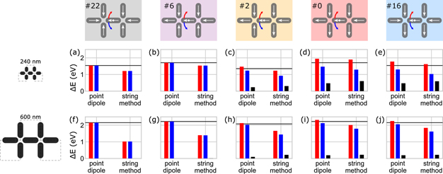
Figure 4. Comparison of switching barriers, for (a)–(e) exchange-dominated and (f)–(j) magnetostatic-dominated square ice and different environment states, as illustrated on top. The schematics on the left show the geometries drawn to scale. For each configuration the clockwise (red bars) and counter-clockwise barrier (blue bars) as well as their difference (black bars), obtained from point-dipole calculations (left) and string-method simulations (right), are plotted. Switching barriers from the simplified point-dipole picture of uniform reversal systematically overestimate the micromagnetic simulation results (i.e. comparing coloured bars), as well as underestimate the amount of barrier splitting for clockwise and counter-clockwise reversal (i.e. comparing black bars). In general, the average point-dipole barrier, indicated with a black horizontal line, is an inadequate approximation to the switching barriers.
Download figure:
Standard image High-resolution imageThe macrospin model considers variation of the single-moment barrier ΔEsb (calculated from the shape anisotropy of a uniformly-magnetised nanomagnet  ) due to point-dipole-like interactions quantified by
  , as derived in section 1.2. We also plot the mean-field barrier from equation (5) (black horizontal line).
The chiral barriers from the string-method simulations are calculated from the energy difference between the micromagnetic net energies of the metastable barrier configuration (↑, ↓) and the initial configuration (←):


For the exchange-dominated square-ice geometry, figures 4(a)–(e), the mean-field barrier always overestimates the lower of the two micromagnetic barriers (for the chosen cases corresponding to counter-clockwise reversal marked in blue), as already discussed in our previous work [15]. Compared to the point-dipole model, micromagnetic simulations consistently give lower chiral switching barriers. The difference of the barrier energies, i.e. the chiral splitting, is enhanced, and remains proportional to the perpendicular moment  generated by the environment. The reversal process is still governed by an almost-coherent rotation of the central moment (appendix
  and stronger interactions
  (appendix
For the magnetostatic-dominated square-ice geometry, figures 4(f)–(j), the differences are even more pronounced. This is because the reversal behaviour is no longer uniform, as discussed in appendices  (black and purple) non-coherent reversal modes are promoted by C- or onion-like magnetic microstates in the central switching nanomagnet [25–28]. This leads to large reductions of the switching barrier, e.g. more than −50% in the case of state #22 in figure 4(f), when compared to the point-dipole model. In contrast, environments with M⊥ ≠ 0 favour S-like micromagnetic configurations associated with quasi-coherent reversal [38–40]. Further details about the micromagnetic switching are discussed in appendix
In general, the point-dipole barriers overestimate all micromagnetic barriers by a considerate margin, and underestimate the chiral barrier splitting, as is evident when comparing the black bars shown in figures 4(h)–(j). For environments with a finite perpendicular magnetisation the barrier splitting is of similar magnitude, figures 4(h)–(j), and thus does not follow the proportionality  . Therefore, the simplified decomposition of switching barriers according to equation (9) is no longer valid when the moments can switch via non-coherent reversal mechanisms.
In general, by taking into account the micromagnetic nature of the moment reversal, we observe both a reduction of the switching barriers as well an enhanced separation of the chiral barriers for environments with  . These results hint to the fact that barrier reductions often utilised in simplified models to simulate the evolution of artificial spin ices [7, 8], and which are often attributed to extrinsic causes such as nanofabrication imperfections, could be—at least partially—associated with intrinsic barrier splitting and incoherent reversal modes.
As lower barriers are easier to overcome for thermally-induced reversal, we therefore expect significant enhancement of the kinetics of artificial square ice, which may yield different relaxation time scales and emergent correlations.
3. Transition kinetics
The effect of barrier splitting on the net transition rate can be generalised by using an average barrier

and a factor f, which describes the symmetric splitting of the clockwise and counter-clockwise barriers around the average barrier, as depicted in figure 5(a),

For the barriers derived from the point-dipole picture in section 1.2, the average barrier corresponds to the mean-field barrier of equation (5), i.e.  . The splitting factor vanishes, f = 0, for environmental states without a perpendicular magnetisation
  acting on the switching moment. From the results of micromagnetic simulations discussed above we obtain non-zero values of f between a few percent up to about 20%.
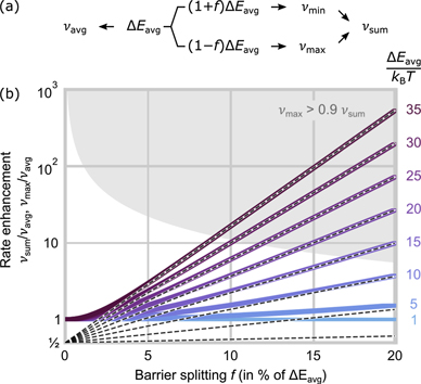
Figure 5. Rate enhancement due to barrier splitting. (a) Via the Arrhenius law, the transition rates νavg, νmax and νmin can be derived for the different barrier energies. (b) The sum rate νsum = νmax + νmin of the two parallel relaxation channels can be significantly enhanced compared to the rate expected from overcoming an average barrier νavg, shown by the solid lines indicating νsum/νavg. The colours denote different kinetic regimes given by the ratio of the average barrier ΔEavg compared to the thermal energy kB T, as indicated by the numbers on the right. Dashed lines denote the respective rate enhancement νmax/νavg associated with transitions via the lower barrier only, which underestimates the rate by a factor of two in the limit of f → 0. Within the shaded area νmax exceeds 90% of the net rate νsum. The rate enhancement is particularly large for rare events where the reduced energy, as indicated by the numbers on the right, is large, i.e. ΔEavg/kB T ≫ 1. It hardly matters, however, in the limit of superparamagnetic fluctuations where ΔEavg/kB T → 1.
Download figure:
Standard image High-resolution image3.1. Modified Arrhenius law for barrier splitting
The temperature-dependent transition rate for spontaneous switching over an average energy barrier ΔEavg can be obtained via the Arrhenius law [41, 42], with the attempt frequency ν0 and the Boltzmann constant kB = 8.62 × 10⁻⁵ eV K−1:

The attempt frequency ν0 depends on the shape, size, and material of the nanomagnets. Typical values of ν0 are in the order of 109...12 Hz [42, 43], and even faster time scales have been discussed [44, 45].
We need to consider the clockwise and counter-clockwise reversal as parallel and independent channels of relaxation, and the rates associated to each of the two barrier energies, i.e. ΔEavg(1 − f) and ΔEavg(1 + f), need to be added to obtain an effective transition rate. Therefore, for the definition of the rate in equation (15), we explicitly included a pre-factor of two, to account for degenerate clockwise and counter-clockwise relaxation channels over the average barrier.
Due to the pronounced non-linearity of the Arrhenius law, the summation of rates leads to an effective increase of the net transition rate νsum of thermally-activated switching when compared to the rate νavg associated with the average barrier (derivation in appendix

The ratio of the joint rate compared to the average-barrier rate, i.e. νsum/νavg, are compared in figure 5(b) for different splitting ratios f and reduced energies ΔEavg/kB T. The exponential rate enhancement is particularly pronounced in the limit of rare events with ΔEavg/kB T ≫ 1 where a splitting of barriers can increase the (albeit low) transition rates by several orders of magnitude (purple lines). In contrast, in the limit of superparamagnetic fluctuations, i.e. ΔEavg/kB T → 1, barrier splitting increases the net rate only moderately (blue lines).
For the assumption that transitions occur predominantly via the lower barrier only, we have to consider the transition associated to the smaller barrier, i.e. (1 − f)ΔEavg, see dashed lines in figure 5 giving the ratio νmax/νavg. For high splitting ratios f and ΔEa
/(kB
T) ≫ 1 the rate νmax will approach νsum, as transitions by the higher-lying barrier become irrelevant. The shaded area of figure 5 marks where νmax exceeds 90% of the value νsum. Within this regime, transitions via the lower-lying barrier might be a good approximation of the net reversal rate. In the limit of f → 0, however, where both barriers are equal, using the rate νmax will underestimate the net rate by a factor of two, i.e.  .
.
In the case of artificial square ice, and depending on the kinetic regime given by the relation between the energies ΔEsb, JNN, and kB T, approximating the transition rates via the mean-field barrier [7, 8, 13, 37] or the minimum barrier [46, 47] thus may significantly underestimate the speed of evolution.
3.2. Temporal evolution of extended square ice
To illustrate the consequences of barrier splitting, we now turn to the evolution of extended square-ice arrays. In many thermal relaxation studies of artificial spin ice, the main interest lies in the onset of phase transitions and formation of emergent correlations. In many experiments, the system evolves from a field-set fully magnetised state, for which we predict a particularly strong barrier splitting. We therefore expect that the initial demagnetisation of a magnetic-field-saturated artificial square ice array will be particularly affected by the modified transition kinetics.
To model the relaxation, kMC simulations are often employed [48–50]. The kMC algorithm provides a numerical solution to the master equation, which is a system of linear differential equations describing the evolution of the probabilities for Markov processes in systems that jump from one state to another in continuous time [51]. Using this method, both the equilibrium expectation values of populations and their dynamical evolution during a thermalization process can be retrieved.
In this work, kMC simulations are performed using a custom-written code [52], with a system of 50 × 50 moments and periodic boundary conditions. The initial configuration is uniformly-magnetised, with the net magnetisation being parallel to a diagonal direction of the array. The demagnetisation due to spontaneous moment reversals is tracked over time for 125 × 103 kMC steps, and averaged over 20 individual simulation runs. As an illustrative example, we here consider the effect of symmetric barrier splitting only, and discount further barrier reductions associated to non-uniform reversal. Thus, we use the point-dipole energy barriers from figure 3(b) with parameters  0.178 eV and ΔEsb = 1.327 eV (i.e. using values for the exchange-dominated square-ice geometry), and calculate the environment-dependent transition rates νavg and νsum at a temperature of T = 300 K as input parameters for the kMC simulations.
Figure 6(a) compares the time evolution of the net magnetisation of square ice for rates from the mean-field barriers (dashed black line) to the model taking into account chiral barrier splitting (solid red line). The time is measured in multiples of the inverse attempt frequency,  . We find that the onset of demagnetisation for the split-barrier model (red) happens two orders of magnitude earlier than for the average-barrier model (black). In the case of the average-barrier model, the demagnetisation involves bouts of rapid evolution interrupted by phases with little change, indicating avalanche-like dynamics [53–56]. In contrast, the split-barrier model shows a smooth demagnetisation, with a rate (solid thick lines indicate evolution from from 90% to 50%) which is about three orders of magnitude faster compared to the mean-barrier model.

Figure 6. Evolution of extended square ice from kMC simulations using point-dipole barriers calculated for the exchange-dominated geometry. (a) Time-dependent net magnetisation, using switching rates obtained from the mean-field (dashed black line) and split-barrier model (solid red line). The time axis is normalised to the characteristic time scale given by the inverse attempt frequency  . For the split-barrier model, the onset and rate of demagnetisation happens earlier and faster when compared to the mean-field-barrier model. (b) and (c) Snapshots of spatial configurations for the (b) mean-field and (c) split-barrier model. Pixels correspond to four-vertex spin arrangements. Those featuring a diagonal magnetisation or a ground-state configuration, are marked in gray or blue, respectively.
Download figure:
Standard image High-resolution imageWhen assessing the emergent spatial correlations, we find that the evolution for the mean-field model is governed by the propagation of strings of ground-state vertices (in blue) wrapping the system (due to the periodic boundary conditions), as shown in figure 6(b). The final state has a magnetisation of about 16% of its initial value. The snapshots of spatial configuration of the split-barrier model at M = 0.9 and M = 0.5 (with M normalised to the initial field-set magnetisation) in figure 6(c) appear somewhat similar to that of the mean-field case. There are more possible transitions for the system to explore, and we would like to point out that this model recovers the separation of strings observed in experiments, but does not require to invoke external disorder e.g. via variation of the switching barriers as done in [8]. The final state of the evolution corresponds to a multi-domain state with almost vanishing magnetisation, M ≈ 0.
Thus, our kMC results show that the modified hierarchy of transition barriers due to the chiral barrier splitting may have subtle, but relevant, consequences: in certain cases, the kinetic relaxation pathways are not simply dictated by equilibrium-energy arguments. This will modify the emergence of spatial correlations, which needs to be explored in a systematic study and compared to experimental results [1, 9, 10, 53, 57–64].
4. Conclusions
To realistically model the temporal evolution of artificial spin ices or small-scale nanomagnetic circuits it is necessary to know the switching barriers for the single-moment reversal. In this work, we quantified how magnetostatic interactions with neighbouring nanomagnets modify the switching barriers in artificial square and kagome ice in absence of extrinsic effects such as defects or spurious fields. We found that for environments which feature a finite perpendicular magnetic field acting on the switching nanomagnet clockwise and counter-clockwise moment reversals need to be considered independently. The resulting barrier splitting can be sizeable. In the case of exchange-dominated nanomagnets supporting coherent rotation modes, the splitting can be predicted from a modified point-dipole model. Taking into account the finite size of the nanomagnets and the influence of material parameters, further barrier reductions were obtained from micromagnetic simulations. These reductions are particularly strong for magnetostatically-dominated nanomagnets embedded in environments that do not promote reversal via a distinct chiral switching channel.
The splitting and reduction of transition barriers exponentially increase the transition rates when compared to a mean-field average barrier. Depending on the dynamical regime, which depends on the relationship between the average energy barrier, barrier splitting and temperature, we found that transition rates are especially enhanced in the limit of rare events. We modelled the evolution of extended artificial square ice with kMC simulations, and compared a mean-field model with the model that takes into account the barrier splitting. We found that the onset and speed of evolution is largely enhanced in the latter case. Furthermore, while mean-field barriers are solely dictated by equilibrium-energy arguments, the chiral switching barriers depend on the kinetics of reversal. Thus, more and different relaxation pathways are accessible, which modifies the emergent spatial correlations and routes towards the ground state.
Our results are a step towards a deeper understanding of the single-moment switching of nanomagnetic systems, highlighting how faster time scales of relaxation can be caused via intrinsic interactions with the magnetic environment. These findings are relevant to the field of artificial spin systems, and can be extended from square ice to other moment configurations, such as kagome ice [6, 53, 54, 65], and square-ice-like tetris, shakti, and brickwork lattices featuring asymmetric moment coordinations [66–68]. We also expect that these concepts are relevant for the utilisation of magnetic metamaterials for magnonics [39, 69–74] and nanomagnetic computation [13, 37, 47, 75, 76].
Acknowledgments
MP gratefully acknowledges David De Sancho for the assistance during the development of the kMC simulation code. The computational results presented have been in part achieved using the Vienna Scientific Cluster (VSC). NL has received funding from the European Union's Horizon 2020 research and innovation programme under the Marie Słodowska Curie Grant Agreement No. 844304 (LICONAMCO). NL, MM, and PV acknowledge support from the Spanish Ministry of Economy, Industry and Competitiveness under the Maria de Maeztu Units of Excellence Programme (MDM-2016-0618), and the Spanish Ministry of Science and Innovation funding the pre-doctoral Grant PRE2019-088070 and the project RTI2018-094881-B-I00 (MICINN/FEDER). KH acknowledges funding by the Swiss National Science Foundation (Project No. 200020_172774).
Data availability statement
The data that support the findings of this study are available upon reasonable request from the authors.
Appendix A.: Derivation of point-dipole barriers
We assume that all moments are strictly parallel (←, →) to the nanomagnet long axis, and that the environment nanomagnets remain static during the reversal of the central moment. We furthermore assume that the configuration of highest energy correspond to those with perpendicular central moment (↑, ↓). These approximations are valid for weak interactions only, and in general are a gross oversimplification, as due to the pairwise couplings the macrospins may rotate away from the local symmetry axis. This would result e.g. in non-symmetric splitting for clockwise and counter-clockwise transitions (i.e. Δϕ ≠ π). Nevertheless, the strict limitation of moment direction allows to employ the anti-symmetry of the dipolar interaction energy under moment rotations of π,

The mean-field barrier  is the average of clockwise and counter-clockwise energy barriers. Under the above assumptions, and as derived in appendix B of reference [15], it is determined by ΔEsb and the energy difference between the equilibrium states before and after switching. It does not depend, however, on the energies of the intermediate high-energy configuration.
The barrier splitting  between clockwise and counter-clockwise rotation, see equation (9), can be calculated from the energy difference of the high-energy states. Using the anti-symmetry argument of equation (A.1), i.e.
  , one obtains

Here,  takes into account the dipolar interaction terms with the central moment only as couplings between other moments remain unchanged by the reversal, and thus fall out of the energy difference.
As shown in figure A.1(b), in the high-energy state interactions with the horizontal nanomagnets, i.e. moments 5 and 6 in figure 1(b), will vanish as  . Due to the staggered arrangement of the moments, a ferromagnetic head-to-tail alignment of the central nanomagnet to its perpendicular neighbours is favourable, whereas the opposite orientation is penalised, see figure 1(c). Thus, only the net perpendicular magnetisation
  is relevant to the splitting. With a modified pair-wise interaction
  one obtains

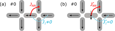
Figure A.1. Definition of interactions JNN
and  . Nearest-neighbour dipolar interactions for (a) the equilibrium and (b) the high-energy configuration. In the latter, the staggered arrangement of moments gives rise to a preferred ferromagnetic head-to-tail arrangement in the excited configuration, with a modified dipolar nearest-neighbour interaction strength
  . Interactions of the central moment with horizontal moments via
  vanishes.
Download figure:
Standard image High-resolution imageAppendix B.: Arrhenius law for barrier splitting
If the transition barriers split symmetrically by a fraction f around the average barrier ΔEavg to values ΔEcw/ccw = (1 ± f)ΔEavg, the joint effective rate νsum = νcw + νccw can be expressed as follows:


Here, C = ΔEavg/(kB
T) denotes the reduced average switching energy barrier. We assume that the attempt frequencies ν0 are independent of the energy of the saddle point, i.e.  . The transition rate νavg(ΔEavg, T) is defined in equation (15).
The maximum of the clockwise and counter-clockwise switching rates is associated to the lower-lying energy barrier (1 − f)ΔEavg. In the limit of f → 0, νmax is a factor of two smaller than the rate νsum(f = 0), and approaches the value of νsum for large splitting f or large reduced energy C ≫ 1:


Appendix C.: Additional simulation results
C.1. Magnetisation during reversal
To quantify the uniformity of the magnetic reversal, figure C.1 shows the averaged moments for a single (non-interacting) nanomagnet and each of the representative double-vertex configurations presented in figure 4. Here, the average magnetisation of each nanomagnet is plotted for every step of the string-method minimum-energy path. The horizontal coordinate roughly corresponds to the rotation angle ϕ of the central moment, with end points denoting initial and final equilibrium states.

Figure C.1. Variation in magnetisation during moment reversal for (a) exchange- and (b) magnetostatic-dominated square-ice geometries. Plotted are the average magnetisation of an isolated nanomagnet (left) and of the individual nanomagnets obtained from the minimum-energy path simulations for each of the representative configurations in figure 4. The average moment Mx along the horizontal (i.e. parallel to the easy axis of the central nanomagnet) and My along the vertical direction are plotted in red and blue, respectively. Values for clockwise (counter-clockwise) rotation from left to right are plotted by thick (thin) lines. The average net moment |M| of each nanomagnet is indicated by magenta lines (note the reduced scale annotated on the left of the isolated nanomagnet).
Download figure:
Standard image High-resolution imageIn general, we find that in equilibrium the net moment |M| (magenta lines) is very close to one. Therefore, the static nanomagnets assume an almost saturated configuration, with the magnetisation largely aligned with the long axis of the nanomagnet and limited edge bending (Mx
, red lines). Interactions with neighbouring moments, however, can induce sizeable perpendicular moment contributions (Mx
⊥ My
, blue lines) in environments that feature a finite perpendicular magnetisation  , i.e. configurations #0, #2, and #16.
In the case of the geometry with small nanomagnets dominated by exchange interactions the magnitude |M| remains largely constant, figure C.1(a). The reversal thus represents a quasi-uniform rotation of the central moment. During reversal, the magnetisation components of the neighbouring nanomagnet can vary, allowing the system to evolve via the most efficient pathway.
For the geometry with large nanomagnets dominated by magnetostatic energy, shown in figure C.1(b), the switching of the non-interacting nanomagnet (left) involves a reduction of the net moment to 91%, and thus does not conform to a uniform moment rotation. For environment states #0, #16, and #2 with  the reduction of net magnetisation is similar to that of an individual nanomagnet. In contrast, for environment states #6 and #22, with
  , we observe a pronounced reduction of magnetisation in the high-energy configuration to less than 70% of the net moment. This indicates reversal via non-coherent modes, which are favoured to occur in nanomagnets that conform to C- or onion-like magnetic microstates promoted by the order of the surrounding nanomagnets [38–40]. This leads to a reduction of the switching barrier as well, as discussed in section 2. The magnetic configuration of neighbouring nanomagnets varies less during reversal when compared to the small-island geometry. This is because the relative volume fraction of the large magnets meeting at the vertex point, where the spin structure varies the most, is smaller.
C.2. Micromagnetic barriers
The switching barriers obtained from micromagnetic string-method simulations for the environment states #0-#31 are summarised in figure C.2 with (a)–(c) showing the results for the exchange-dominated, and (d)–(f) the magnetostatic-dominated geometry.
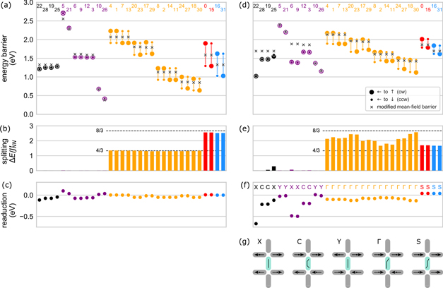
Figure C.2. Switching barriers from micromagnetic string-method simulations, for (a)–(c) exchange- and (d)–(f) magnetostatic-dominated square-ice geometries. (a) and (d) Barrier energies for the moment reversal from left to right via clockwise and counter-clockwise pathways (large and small circles, respectively). The modified mean-field barrier, discussed in appendix C.2, is marked with a cross. (b) and (e) Difference of the two barriers, compared to the modified mean-field prediction of the barrier splitting (dashed lines). (c) and (f) Difference between the modified mean-field barrier (marked by crosses in (a) and (d)) and the average micromagnetic barrier of clockwise and counter-clockwise reversal (i.e. centre of vertical lines in (a) and (d)). Large differences are observed especially for those environments which do not promote transitions of preferred chirality (marked in black and purple). (g) Nomenclature of the environment states used in (f), determined by the relative orientation of the perpendicular nanomagnets. The configuration of the neighbouring nanomagnets promotes edge bending of the micromagnetic configuration, which affects the mechanism of moment reversal and thus can lead to additional barrier reductions.
Download figure:
Standard image High-resolution image
We compare the clockwise and counter-clockwise barriers, large and small circles in figures C.2(a) and (d), to a modified mean-field model. The predictions are based on equations (5) and (9), but instead of energies derived from point-dipole calculations we use those obtained from micromagnetic simulations, as follows:
First, the switching barrier ΔEsb of an isolated nanomagnet simulated with the string-method is used, as opposed to the shape anisotropy calculated for a uniformly-magnetised nanomagnet. For the exchange-dominated nanomagnet geometry we obtain  1.540 eV compared to
  1.327 eV, which is a reduction of -14%. For the magnetostatic-dominated nanomagnet geometry, the barrier reduction is even bigger, with
  2.153 eV and
  1.691 eV (−22%), as the reversal is no longer coherent (see figure C.1(b)).
Second,  and
and  correspond to the micromagnetic equilibrium energies of the static configurations. Together with
  , a modified mean-field barrier can be calculated from equation (5) (crosses in figures C.2(a) and (d)).
Third, to estimate the barrier splitting, the nearest-neighbour interaction  is rescaled. The rescaling is motivated by the point-dipole model, which predicts an energy difference of
  between the lowest-lying ground state and highest monopole state:

For the exchange-dominated small-island geometry we find that the modified mean-field barrier gives a passable estimate for the average switching barrier, as the small differences in figure C.2(c) show. The chiral barrier splitting is well-described by the rescaled energy  , albeit with a small reduction for fully-magnetised environments marked red and blue in figure C.2(c).
For the magnetostatic-dominated reversal in the large-island geometry, figures C.2(d)–(f), the mean-field approach fails: the barrier splitting is both overestimated for environments with  (red and blue) as well as underestimated in the case of
  (yellow). In particular, the mean-field barrier predictions fails for environments with
  (black and purple), where reversal via non-uniform modes are favoured, as discussed before. The reductions compared to the mean-field barrier seem to be particularly strong for environments which feature 'X' and 'C' configurations of the perpendicular moments, see figures C.2(f) and (g). The symmetry breaking by the environment promotes so-called onion or C- microstates in the central nanomagnet, respectively [38–40]. These states promote non-coherent reversal, as illustrated in supplementary material figure 2, and a reduction of the switching barrier, as discussed in figure C.1 and appendix C.1.
With the exception of  , which is a result of the string-method simulation, the energies
  and
and  can be obtained from static equilibrium micromagnetic simulations, e.g. using OOMMF [21] or MuMax3 [22]. This makes this approach attractive to estimate more realistic switching barriers based on a perturbative decomposition of a single-nanomagnet behaviour plus a correction term due to interactions with the neighbouring moments. This approach seems valid for relatively small nanomagnets favouring reversal via uniform modes, but fails if more complex reversal mechanisms are accessible.