


Abstract
We consider the use of quantum-limited mechanical force sensors to detect ultralight (sub-meV) dark matter (DM) candidates which are weakly coupled to the standard model. We show that mechanical sensors with masses around or below the milligram scale, operating around the standard quantum limit, would enable novel searches for DM with natural frequencies around the kHz scale. This would complement existing strategies based on torsion balances, atom interferometers, and atomic clock systems.
Export citation and abstract BibTeX RIS
1. Introduction
There is overwhelming astrophysical and cosmological evidence for the existence of cold dark matter (DM) [1–4]. However, the detailed properties of the DM, in particular its mass, are highly unconstrained [5]. The possibility that the dark sector could contain or even consist primarily of 'ultralight' bosonic fields of mass 10−22 eV ≲ mϕ ≲ 0.1 eV has recently received considerable attention [6–8].
The existence of such light fields coupling to the standard model (SM) may induce new forces beyond the usual electroweak and strong forces. For example, if there are additional light scalars which couple to SM matter through Yukawa couplings, the best constraints come from torsion balance experiments looking for '5th forces' between a pair of macroscopic masses [9, 10]. Furthermore, as first emphasized in [11], if these ultralight bosons make up a significant fraction of the ambient DM background, existing mechanical accelerometers [9, 10, 12, 13] and upcoming large-scale atomic interferometers (eg. [14]) can be used to further probe these models.
Ultralight DM detection can be viewed as a paradigmatic exercise in quantum metrology. Essentially, the dark matter creates a classical, persistent, but extremely weakly-coupled force on a sensor. The goal is to then detect or rule out the presence of this force. This task is fundamentally limited by the noise in the detection system. High-quality microwave cavity systems are already used for such metrological searches for a particular ultralight DM candidate—the axion, which couples to the electromagnetic field in the cavity [15, 16]. Here we instead focus on ultralight DM candidates which couple to all atoms in a massive object coherently, for example through direct coupling to neutron number.
In this paper, we study the prospects for searching for these ultralight DM candidates using massive, mechanical sensors. These devices consist of optical or microwave fields optomechanically coupled to a diverse range of mechanical systems, including suspended pendulums [17–19] and torsion balances [9, 10], high-tension mechanical membranes [20, 21], levitated dielectric [22–25] or magnetic [26–28] objects, and even levitated liquids [29]. Our primary goal is to understand the parametric scalings in sensitivity with a variety of systems of different masses, frequencies, and noise levels, rather than to focus on a specific experimental setup. This complements the detailed analysis based on the Eötvös–Washington experiments presented in [11].
We emphasize the utility of multiple sensing devices (in an array or distributed at widely separated locations) for DM detection. Arrays of sensors benefit from reduction of the noise compared to the correlated DM signal, and enable rejection of some important backgrounds. In particular, the signals we consider here act differently on different material types, unlike the gravitational and seismic noise backgrounds dominating at low frequencies. Thus an array with at least two different types of material sensors can be used to make differential measurements which subtract out these backgrounds [11]. We will see that at the level of a pair of sensors in a well-isolated environment (eg. dilution refrigeration) these mechanical sensors already have detection reach competitive with existing torsion balance and interferometery experiments. Arrays of Ndet sensors can further enhance the detection reach by a factor of at least  , and as fast as Ndet, in the case of correlated, 'Heisenberg-limited' readout [30]. We find that optomechanical systems are well-poised to contribute to searches for ultralight DM for masses below around 10−8 eV; for higher masses the laser power requirements in the readout become very stringent (see figure 4). Detection frequencies in the kHz–MHz range appear to be the most promising.
Recently, it has been proposed that a large array of mechanical sensors operating with significant quantum noise-reduction could enable direct detection of heavy (m ≳ mpl) DM candidates purely through their gravitational interactions [31]. Here, we propose ultralight DM detection as a nearer-term goal achievable with just a few mechanical sensors, operating at noise levels around the 'standard quantum limit' (SQL), a benchmark already demonstrated in many devices. The scalable nature of an array and potential improvements to the noise levels beyond the SQL would allow for significant ultralight DM detection reach en route to the long-term goal of gravitational DM detection with mechanical sensors.
2. Ultralight DM
To begin, we briefly review the salient facts about ultralight DM. The essential feature of these ultralight candidates is that they behave as a persistent, wave-like field, due to their high occupation number. This should be contrasted to heavier DM candidates, for example GeV-scale weakly interacting massive particles (WIMPs), which manifest as a dilute gas of single particles. See [32] for a general review of DM properties, and [8, 33] for reviews of ultralight DM.
Suppose the dark sector consists of a single bosonic field of mass mϕ . Bosonic DM is required to have mϕ ≳ 10−22 eV so that its de Broglie wavelength does not exceed the core size of a dwarf Galaxy and to satisfy Lyman-α constraints [7, 34–36] (note that recent evidence indicates that the constraints may be a few orders of magnitude stronger than this [36–38]). DM this light is necessarily bosonic as fermionic DM with a mass ≲keV would not fit inside of a dwarf Galaxy due to the Pauli exclusion principle [39]. Assuming that the DM has virialized to the Galaxy, it will be moving with a typical speed v ∼ 105 m s−1 due to the viral theorem, and thus have de Broglie wavelength of order λ = 1/mϕ v 5
Consider the number of DM quanta in a typical cell of phase space. If nDM = ρDM/mϕ is the number density of DM, the phase space occupancy is given by

where the observed value of the local DM density ρDM ∼ 0.3 GeV cm−3. Thus for any mϕ ≲ 0.1 eV, this occupancy is huge, indicating that the DM can be treated as a classical field, essentially a superposition of many different plane waves. These waves have velocities following a Boltzmann distribution. The phases in these plane waves are uncorrelated from each other. Their propagation directions (and polarization vectors, for vectorial fields) are distributed isotropically as long as DM has fully virialized. Superposing a large number of such waves will produce an overall time-dependent waveform with frequency ω ≃ mϕ and frequency spread δω ≈ v/λ = v2 mϕ . This frequency spread leads to a coherence time Tcoh ≈ 1/δω ≈ 106/ω. For a time duration smaller than Tcoh, the DM background field can be approximately treated as a coherent sinusoidal wave with signal angular frequency and wavelength

In figure 2, we give a visualization of the power spectral density (PSD) of the DM field, generated by simulating a large number of superposed DM quanta (see appendix

Figure 1. Schematic of a single-sided cavity optomechanics search for ultralight DM. Photons reflected off the suspended mirror pick up phases proportional to the mirror's position x(t). This information is then read out via standard interferometry. The ultralight DM produces an essentially monochromatic force with wavelength much longer than the size of the sensor; the presence of this force can then be inferred by reading out the cavity light. In this setup with a single sensor, the fixed reference mirror and movable sensor mirror should be made from different materials, as discussed near equation (4).
Download figure:
Standard image High-resolution imageAssuming there is a non-zero coupling between the DM field and the sensor, if the observational time Tint is much shorter than Tcoh, we can parametrize the force exerted on the sensor (along a given axis) by the DM as

under the assumption that the wavelength (2) is much larger than the size of the sensor. In equation (3), g is a dimensionless coupling strength depending on DM model,  , and Ng
is the number of total charges in a given sensor. For example, consider the case that the light boson is a vector boson which couples to neutrons (studied in detailed in the next subsection); then
, and Ng
is the number of total charges in a given sensor. For example, consider the case that the light boson is a vector boson which couples to neutrons (studied in detailed in the next subsection); then  is approximately the number of neutrons in a sensor of mass ms. For observational times longer than Tcoh, we essentially have Nbins = Tint/Tcoh independent realizations of (3), with randomly oriented amplitude and phase.
To get a sense of the force scales involved, consider (3) with g ∼ 10−22 (see figure 4). This would generate a force per neutron of around 10−38 N. This would then be detectable with a second of integration time, using a μ
g-scale device with force sensitivity in the zepto-Newton regime  , for example [40].
The force (3) is proportional to the mass of the sensor, and is thus somewhat analogous to a gravitational force. However, crucially, the constant of proportionality is material-dependent. In the neutron-coupled example, two materials with different neutron-to-nucleon ratios will experience a differential force. This is a general feature of these types of dark matter—they generate 'equivalence-principle violating' forces, as emphasized in [11]. If the force had satisfied the equivalence principle (EP), then the mechanical element of a sensor and whatever its position is referenced to would both experience the same force, and no motion would be detected (one would have to detect the gradient of the force, i.e. the tidal force, see for example [12]). However, these EP-violating forces can be detected directly using a sensor and reference (possibly a second sensor) with different material properties. For example, if the neutron-to-nucleon number ratio of each material is Z1/A1, Z2/A2, then the differential acceleration on the two objects is given by [11]

For typical lab materials, Δ ≲ 0.1.
Aside from the general properties just mentioned, there are several distinguishing features of the signal that can be used to distinguish from background. The first is that the signal has a uniform direction over timescales of the coherence time. This means that force sensors in different directions can be used to isolate the signal while rejecting background. The second property is that the Earth's motion in the Galaxy and self rotation select a preferred direction for signal. More explicitly, the Earth is moving at speed v ∼ 105 m s−1 around the center of the Galaxy. Additionally, there is increasing evidence that there is a stream of non-virialized DM moving past the Earth with velocities also v ∼ 105 m s−1 [41–43]. Thus while it is difficult to say for certain what direction any preference would be, it is certain that the signal will be  biased in some direction. The third is that there will be modulations. The Earth is moving around the Sun at δ
v ∼ 104 m s−1 and the surface of the Earth rotates around its axis as a speed δ
v ∼ 100 m s−1. Thus the DM signal will move fractionally in frequency space by an amount
vδ
v ∼ 10−7 − 10−9.
6
The fourth is that if mϕ
≲ 10−9 eV, the coherence length of DM reaches the size of the Earth, so experiments on multiple parts of the planet would be correlated.
biased in some direction. The third is that there will be modulations. The Earth is moving around the Sun at δ
v ∼ 104 m s−1 and the surface of the Earth rotates around its axis as a speed δ
v ∼ 100 m s−1. Thus the DM signal will move fractionally in frequency space by an amount
vδ
v ∼ 10−7 − 10−9.
6
The fourth is that if mϕ
≲ 10−9 eV, the coherence length of DM reaches the size of the Earth, so experiments on multiple parts of the planet would be correlated.
Our general parametrization (4) can be used to model the signal produced by a variety of DM candidates to produce a basic sensitivity estimate. Here, we briefly exhibit a pair of DM models to show how this type of signal arises.
2.1. Vector B − L DM
The first case we consider is when dark matter is a spin-one particle, which couples to a conserved current. In the SM, there are two conserved currents that a vector-like DM can couple to without introducing new gauge anomalies: electric charge, and baryon number minus lepton number, i.e. B − L charge. For the case of electric charge, DM induced force is highly suppressed since the test objects are generically charge neutral, thus we consider the case where DM is a vector field that couples to B − L charge.
The Lagrangian in this case can be written as

Here n is the neutron field, so the vector boson couples directly to the number of neutrons. The boson mass term can be generated by Higgsing the U(1)B−L group, providing the mass mϕ . For simplicity, the Higgs boson is assumed to be much heavier than the gauge boson, i.e. the Stueckelberg limit. The vector gauge boson is assumed to couple to B − L charge. For a charge neutral test object, Aμ effectively couples to the total neutron number.
Taking the Lorentz gauge, i.e. ∂μ
Aμ
= 0, one can show that A0 is smaller than Ai
by a factor of the velocity of dark matter, v ∼ 10−3. One also finds that the dark electric field is much larger than the dark magnetic field, i.e.  . In the plane wave approximation, the dark electric field can be written as

where the normalization is set to reproduce the observed local DM mass density, and the frequency is set by the mass of the DM, i.e. ωϕ ≃ mϕ . This will produce a force of the form

on each sensor. For the frequencies under consideration, the wavelength is much larger than the size of the experiment so that we will drop the x dependence. Here for a sensor with mass ms,  , which is the number of neutrons in the sensor and
  .
.
2.2. Scalar coupling to neutrons
Another option for light DM is that it is a spin-zero particle. It can couple to SM fermions through two types of couplings, derivative and non-derivative interactions. Derivative interactions couples to a vector quantity of the test mass. The test mass tends to have very low intrinsic spin and thus do not couple very strongly to derivative interactions. As such we consider non-derivative interactions.
The leading non-derivative interactions a scalar can have with the SM are Yukawa interactions, much like the well known example of the Higgs boson. Similar to the Higgs boson, in the presence of a coherent background of the light scalar field, these Yukawa interactions have the effect of modulating the mass of a particle. The spatial dependence of the mass results in a force on the test mass.
In order to make a close analogue to the previous example, we imagine a model where the scalar DM ϕ couples only to neutrons through a Yukawa coupling

Under the planewave approximation, the force on an object with Ng neutrons can be written as

Note that this example is similar to (7) except that the two couplings are named differently, gB−L versus y. The only other difference comes from the velocity suppression; in terms of the parametrization (4) here we have g = vy. This is due to the fact that forces are vector quantities and for the case of a scalar, the only vector quantity to provide a direction is the small velocity.
3. Detection with optomechanical force sensors
In this section we give a brief overview of continuous force sensing, with the goal of explaining how force-sensitivity curves are derived in a typical quantum optomechanics experiment. See appendix
Consider a prototypical force sensor consisting of a high-finesse optical cavity formed by a partially transparent mirror on one side and a high-reflectivity mirror suspended as a pendulum of mass ms and mechanical frequency ωs on the other side (see figure 1). The suspended mirror is used as the sensor, which can be monitored by light sent into the cavity through an external laser. Displacements of the mirror x(t) produce changes of the cavity fundamental frequency, leading to a coupling of the light and mechanics. Light emerging from the cavity picks up a phase dependent on the mechanical displacement, which can then be read out via standard homodyne interferometry. Given the observed displacement signal x(t), we can infer the presence of forces F(t) on the sensor using standard linear response theory.
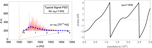
Figure 2. Example simulated PSD and phase drift for vector dark matter of mass mϕ
= 6.6 × 10⁻¹³ eV, corresponding to a signal frequency ω0 = 1 kHz at zero momentum. One can read off the effective quality factor of the DM signal Q ∼ 106, which sets the coherence time of the signal. In terms of the force signal expected on a device, the left plot represents precisely the shape of the force signal PSD, with the scale set by the coefficient in (3). See appendix
Download figure:
Standard image High-resolution imageThe classic example of such an optomechanical setup is LIGO [17]. Here we are describing a simplified version of one of the interferometer arms. The use of mirrors and light is non-essential, however: numerous variants of this idea operate in essentially the same way. Examples include microwave-domain electromechanical systems [20, 21], optically-probed levitated objects [22–25], magnetically-probed and levitated superconducting objects [26–28], and even levitated liquids [29]. See [45, 46] for reviews of these types of systems.
The sensitivity of a given sensor is set by noise. In general, the force acting on the sensor is

where Fsig represents the signal we are looking for and Fnoise is a random force coming from a variety of noise sources. Assuming that the noise is a stationary random variable, the size of the noise is characterized by the noise force PSD SFF , defined by

The noise force PSD has units of force2/frequency. The interpretation of this quantity is that if one wants to detect a signal force of pure frequency ωϕ and amplitude F* at the one-σ level, one needs to continuously monitor the sensor for an integration time Tint given by

The smaller the signal one is looking for, the longer integration time Tint is needed
7
. Sensitivities are usually quoted as the square root of SFF
, say in units of  . The appearance of the square root of frequency reflects the Brownian (stationary) character of the noise.
A number of sources contribute to the noise on a sensor. The two key noise sources we will consider in this paper are thermal noise coming from the coupling of the sensor to its ambient environment as well as measurement-added noise. This latter noise is a fundamental limitation imposed by quantum mechanics: the act of measurement itself induces noise. We write

In what follows, we will study the fundamental limits to detection of ultralight DM imposed by thermal and measurement noise. A key assumption here is the elimination of correlated technical noise sources, such as seismic noise. Methods for achieving this are discussed in section 3.3, see also the appendix
3.1. Thermal noise
Thermal noise here refers to a random Brownian force FT(t) acting on an individual sensor from thermal fluctuations coupling to the environment. In general, this will come from both direct vibrational coupling of the sensor to its support structure as well as residual gas pressure in the sensor. At the frequencies of interest in this paper, these are white (frequency-independent) stationary noise sources. Simple dimensional analysis (see also appendix

Here the first term reflects coupling of the sensor to phonons in its support structure; γ is the mechanical damping rate of the sensor and T is the temperature of the environment. The second term comes from residual gas pressure in the environment, where P is the gas pressure, As is the surface area of the sensor, and ma is the mass of an individual gas molecule.
3.2. Measurement noise and the 'SQL'
Measurement-added noise comes from the quantum mechanics of the act of measurement itself. The measurement noise PSD can be further decomposed into a pair of terms known as shot noise and backaction noise,

In the cavity model given above, backaction noise corresponds to random fluctuations in the input laser amplitude, which causes a random force on the mirror, which is then transduced into the output light. More fundamentally, backaction noise arises as a consequence of the sensor state being measured. Shot noise corresponds to random fluctuations in the input laser phase which then produce a noisy readout 8 .
The backaction and shot noise contributions to the noise PSD are non-trivially dependent on both frequency and readout laser power PL. Backaction tends to dominate at low frequencies while shot noise dominates at high frequencies. Furthermore, as one turns up the laser power, backaction noise increases whereas shot noise decreases. See figure 3 for an example of these noise contributions with a typical mechanical sensor.

Figure 3. Various contributions to the noise PSD of a single sensor, with different input laser powers. Here we have plotted sensitivities for a mechanically-coupled sensor of mass ms = 1 mg, mechanical frequency ωs = 1 Hz, and mechanical damping coefficient γ = 10−6 Hz in a 1 cm optical cavity (parameters based on the setup in [19]). We assume operation at dilution refrigeration temperatures T = 10 mK. The incident laser power in the first row is taken as PL = 1 W and 10−9 W in the left panel and right panel, respectively. The SQL is achieved at the minimum of the total noise curve; the location changes as a function of laser power. In the second row, we show the sensitivity achieved by tuning the laser power to achieve the SQL at each signal frequency ωϕ , for the same sensor parameters (dropping seismic noise for visual simplicity). We see that for these sensor parameters, seismic and thermal noise dominate at low frequencies while measurement-added noise dominates at high frequencies.
Download figure:
Standard image High-resolution imageGiven a target signal frequency ωϕ
that one is looking for, the laser power PL can be tuned to minimize the sum of the backaction and shot noise terms at the frequency ωϕ
. This procedure yields the noise at what is known as the 'SQL', at frequency ωϕ
. See figure 3 for SQL-level force sensitivities. Achieving the SQL at can require substantial laser power at high frequency, see figure 5, which becomes prohibitive for DM masses m ≳ 10−8 eV. As discussed in appendix
For the cavity optomechanics system given above, the total measurement noise for the sensor operating at SQL at frequency ωϕ is given by the simple formula [see equation (B26)]

Here γ is the same mechanical damping rate appearing in (14). Note that this equation is true for force signals only at frequency ωϕ . Achieving the SQL is a frequency-dependent statement: one minimizes the measurement added noise at only the specific frequency ωϕ . The noise power at other frequencies ω ≠ ωϕ is above the SQL. Thus if one wants to achieve the SQL-limited sensitivity over a range of possible signal frequencies, one needs to tune the laser power frequency-by-frequency while scanning over the range. See section 4 for a more detailed discussion of search strategies along these lines.
We emphasize that (16) is true for arbitary signal frequency ωϕ . In particular, this equation holds for signals off resonance with the sensor ωϕ ≠ ωs. It is clear from this equation that a better force sensitivity would come from not only achieving the SQL but also tuning the sensor to be on-resonance ωϕ = ωs, in which case we have

Although tuning the laser power to achieve the SQL over a range of frequencies is in principle straightforward, tuning the actual mechanical resonance frequency is more challenging 9 . One potentially promising avenue would be to use dynamical stiffening techniques, which allow one to increase the effective mechanical frequency by driving the system with laser backaction [47].
Environmental thermal noise is an irreducible floor for any measurement. Although one can lower the temperature, gas pressure, and so forth, any experiment will always have a thermal noise floor set by (14). This is in contrast to measurement-added noise, which can be reduced significantly below the SQL by the use of sophisticated techniques like the use of squeezed readout light [48–51] or quantum backaction-evasion [52–57]. In this paper, we will use the SQL level of measurement noise as a benchmark, but we emphasize that further detection reach is achievable using available post-SQL measurement techniques.
3.3. Detection with an array
All of our considerations above were for a single force sensor. Suppose now that we have an array of Ndet such sensors. The DM signal is now a correlated force acting across the entire array. This provides two key advantages: increasing the signal-to-noise above any uncorrelated noises, as well as offering some routes to elimination of backgrounds and some correlated noises.
Consider first noise sources which act separately on each sensor. For example, we assume that both thermal noise and measurement-added noise, discussed above, have this property. The achievable force sensitivity with an array of Ndet sensors is then simply given by  times the single-sensor sensitivity, because the noises can be averaged out across the array.
The  enhancement comes from assuming that we read out each sensor individually. Further improvement can be made using a coherent readout scheme, in which the same light probes multiple sensors at the same time (note however this will also induce correlated measurement-added noise). In such a scheme, the signal adds at the level of the amplitude, which is then squared to produce the probability we actually read out. In the ultimate case that we use a single light probe to read out the entire array, one can achieve a full Ndet enhancement—the so-called Heisenberg limit in quantum metrology [30].
Use of an array also serves an extremely important purpose beyond increasing the sensitivity: elimination of backgrounds and technical noise. In particular, as emphasized above and in [11], the kinds of signal forces here couple to different materials differently (e.g. the B − L force couples to neutron number). This is much like an EP violating force. If we construct an array consisting of sensors built from two different materials, we can then make differential measurements between the two types in order to remove backgrounds that act identically on all the sensors. Atom interferometers using two atomic species or torsion balance experiments looking for EP violation use this technique to remove seismic noise, which becomes extremely important at low frequencies. Other correlated noise sources can also be suppressed by doing differential measurements of this type. In the following section, we assume that these correlated noise sources have been sufficiently controlled so that thermal and measurement-added noise are dominant.
4. Detection reach and search strategy
In this section, we study the DM detection reach of mechanical sensor arrays. Given a specific sensor, environment, and measurement protocol, we have a noise PSD SFF (ω). For simplicity, we will assume that the entirety of the DM sector consists solely of one ultralight field 10 and take the force of the form in (4). We then obtain a bound on the coupling strength using our force sensitivity (12). All told, with Ndet sensors in the array, our fundamental DM detection reach (i.e. the smallest value of the DM–SM coupling we can detect) is set by

We assume incoherent readout of the individual sensors in the array; as discussed in section 3.3, coherent readout enhances the denominator by another power of Ndet.
In (18), the time Ttot is an effective total integration time. In general, we assume that our sensors can be operated for some integration time Tint set by technical constraints like laser stability, typically on the timescale of hours. There are then two basic DM regimes. Recall that the DM signal is essentially a coherent, monochromatic force on timescales Tcoh ≈ 106/ωϕ with ωϕ = mϕ set by the DM mass. For low frequency DM, we have Tint < Tcoh, so a complete integration run will see a coherent signal. For higher-frequency DM candidates, Tint > Tcoh, so the signal consists of Nbins = Tint/Tcoh bins worth of independent signals. These bins can be summed in quadrature, and so we define the effective integration time

We note that to scan for signals in bins in this fashion will require some use of template matching algorithms, similar to waveform matching used by LIGO. In particular, with sufficiently long integration times, templates will be required to take into account long-wavelength features like the rotation of the sensing setup with respect to the DM direction. While this can present computational challenges with long integration times, it also enables a mechanism for rejection of backgrounds which do not share the same temporal shape as the expected DM signal.
In the following, we consider three basic search strategies:
Single shot search. The simplest 'strategy' would be to simply assume a fixed laser power and integrate for Tint. This produces a sensitivity curve which is best at some particular DM mass mϕ , i.e. a particular signal frequency ωϕ , namely the frequency at which this laser power corresponds to the SQL. For DM masses away from this particular frequency, the resulting sensitivity curve is non-optimal. Some examples are given in figure 4(a).
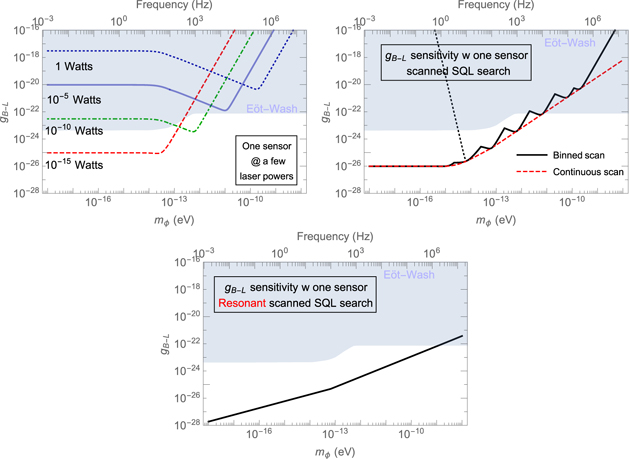
Figure 4. Sensitivity coverage on the DM coupling for various search strategies, using same sensor parameters as in figure 3, using the vector B − L model for illustration. We assume a reference mirror made of iron and moveable mirror made of silicon for concreteness (again based on the setup in [19]), leading to a differential acceleration coefficient Δ ≈ 0.03. Top left: sensitivity curves for the simple search strategy, with a single fixed laser power. Top right: idealized search strategy with sensor tuned to reach the SQL for each target frequency, with fixed mechanical frequency ωs. The jagged curve represents our binned search strategy described in the text. Bottom panel: fundamental limit on detection reach, scanning over resonance frequencies ωϕ
= ωs. In all plots, we only allow for realistic laser powers PL ≲ 1 W as described in appendix
Download figure:
Standard image High-resolution imageSQL scan at fixed mechanical frequency. To do better, one should scan over DM masses by scanning over various values of the laser power, achieving the SQL frequency-by-frequency. Using (16) in (18) and assuming that the dominant thermal noise is from phononic coupling, this corresponds to a sensitivity curve

In figure 4(b), we plot the ideal case in which one achieves the SQL for every frequency; since this is an infinite number of frequencies and we need to integrate for Tint at each, this is only a fundamental limit. A more realistic strategy is also plotted in figure 4(b), in which we bin the DM masses by order of magnitude, and tune the laser to a power optimized once for each bin. For the large span of available light DM parameter space below O(10−8 eV), and an integration time of order 1 h per bin, the full spectrum could be scanned in roughly one day. In each case, we assume a maximum achievable laser power of around 1 W. This means that at sufficiently high DM mass, we are operating at a noise level worse than the SQL (see figure 5).
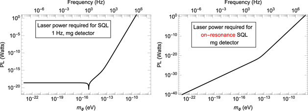
Figure 5. Laser power required to achieve the SQL. Top: fixed mechanical frequency ωs. Bottom: variable mechanical frequency ωs, with SQL achieved on-resonance ωϕ = ωs. Same sensor parameters as in figure 3, and assuming a cavity length L = 0.1 m. We see that at sufficiently high signal frequency, the SQL requires prohibitively large laser power PL ≳ 1 W. In our sensitivity curves, we only allow for laser powers below 1 W; at higher frequencies we are therefore working at noise levels above the SQL.
Download figure:
Standard image High-resolution imageResonant SQL scan. Finally, we consider the ultimate limit of resonant sensors operating at the SQL: a scan in which we vary the mechanical frequency of the sensor to resonance with the DM frequency ωs = ωϕ . From (20) this yields a sensitivity curve

As discussed in section 3.2, this could potentially be achieved (at least over some orders of magnitude in frequency) using dynamical stiffening of a fixed sensor.
Equation (21) can be used to gain some basic intuition about the scaling of the DM detection problem. Note that Ng
∼ ms, so our smallest detectable DM coupling scales like  . Thus the fastest way to win is simply to build a more massive sensor! As discussed in section 3.3, the array approach can do better than simple scaling in the total mass if one has coherent readout of the array, in which case we can achieve a scaling
  . We also see that the overall sensitivity
  , so lower damping rates (i.e. higher Q-factor resonators) can significantly increase our sensitivity. Finally, we can observe a simple crossover behavior: for low frequency signals kT > ωϕ
the thermal noise dominates while for high frequencies kT < ωϕ
, the SQL measurement-added noise dominates. This in particular suggests that backaction-evasion or some other kind of post-SQL strategy will be most beneficial at frequencies ωϕ
≳ kT ∼ 1 GHz (for dilution refrigeration temperatures T ∼ 10 mK).
, so lower damping rates (i.e. higher Q-factor resonators) can significantly increase our sensitivity. Finally, we can observe a simple crossover behavior: for low frequency signals kT > ωϕ
the thermal noise dominates while for high frequencies kT < ωϕ
, the SQL measurement-added noise dominates. This in particular suggests that backaction-evasion or some other kind of post-SQL strategy will be most beneficial at frequencies ωϕ
≳ kT ∼ 1 GHz (for dilution refrigeration temperatures T ∼ 10 mK).
5. Conclusions and outlook
Quantum sensing technology offers a highly promising route to searches for new physics beyond the SM. Macroscopic sensors have already been demonstrated as gravitational wave detectors in LIGO, and development of these technologies should continue to push the precision Frontier forward for years to come.
In this paper, we have suggested a clear target for sensing using mechanical sensing devices: models of DM consisting of very light bosonic fields. If the dark sector contains such a field, it produces a nearly monochromatic force signal on a sensor, precisely the type of signal these sensors are optimized to detect. We have argued that sensors with already-demonstrated sensitivities have non-trivial detection reach in this parameter space. With an array of sensors, one can achieve a rapidly scaling sensitivity to these DM candidates. Since these signals also act different on different materials, the use of at least two material species of sensors can be used to make differential measurements, eliminating many systematic and background errors [11]. In figure 4, we see clearly that mechanical sensors are poised to make a contribution in the kHz–MHz regime, which would provide a complement to atom interferometer and torsion balance approaches operating at sub-kHz frequencies.
Beyond these ultra-light models, quantum-limited force sensing devices should be able to search for many other types of new physics. Since the sensors are macroscopic in size, they should have exquisite sensitivity to any potential signal whose strength increases with the mass of the sensor. Different realizations of the optomechanical force sensing paradigm could be used in complementary ways; for example, magnetic sensors could be used to search for dipole-coupled forces. Ultimately, a large array of these sensors could be able to search for heavy DM candidates purely through the gravitational interaction [31]. This paper presents a first example of a detection target reachable with currently demonstrated mechanical sensing technology, and we hope it encourages further exploration of the potential uses of quantum sensing for physics beyond the SM.
Acknowledgments
We would like to thank Peter Graham, Roni Harnik, Gordan Krnjaic, Konrad Lehnert, Nobuyuki Matsumoto, David Moore, Cindy Regal, and Fengwei Yang for discussions. Special thanks to Jon Pratt for taking and providing us with some benchmark low-frequency seismic noise data. ZL, AH, and YZ would like to thank PITT-PACC, KITP and MIAPP for support from their programs and providing the environment for collaboration during various stages of this work. AH and ZL are supported in part by the NSF under Grant No. PHY1620074 and by the Maryland Center for Fundamental Physics. YZ is supported by US Department of Energy under Award No. DESC0009959. The Joint Quantum Institute is supported by funding from the NSF.
Data availability statement
No new data were created or analysed in this study.
Appendix A.: DM signal PSD
Previously we made a simple estimate for the DM signal as a purely monochromatic force. Here, we give a more detailed discussion on the DM signal PSD if the frequency resolution is better than the intrinsic width caused by DM viral velocity.
The DM signal can be simulated by linearly adding up many freely propagating DM wavefunctions, where each DM wavefunction is described by a planewave. For simplicity, we will describe the case of vector DM where

The polarization vector ( ) and the propagation vector (
 ) are independent to each other. We take both vectors to be isotropic in the Galaxy frame. In the non-relativistic limit,
  and the magnitude of
  follows Boltzmann distribution, i.e.
  . Here v0 ≃ 230 km s−1 and vescape ≃ 325 km s−1. The frequency ωi
is determined by |ki
| through the dispersion relation. The magnitude of
. Here v0 ≃ 230 km s−1 and vescape ≃ 325 km s−1. The frequency ωi
is determined by |ki
| through the dispersion relation. The magnitude of  ,
,  , is the same for all particles and it can be calculated by local DM energy density, i.e. around 0.4 GeV cm−3. Furthermore, ϕi
is a random phase associated to each particle, which runs from 0 to 2π with uniform probability distribution (see [13] for details).
, is the same for all particles and it can be calculated by local DM energy density, i.e. around 0.4 GeV cm−3. Furthermore, ϕi
is a random phase associated to each particle, which runs from 0 to 2π with uniform probability distribution (see [13] for details).
The overall force on a sensor induced by vector DM can be written as

In the lab frame, the force can be decomposed in Cartesian coordinate. However, this frame is moving with the Earth respect to the Galaxy frame. This includes both the motion around the galactic center (vE ∼230 km s−1) as well as the motion induced by the Earth's rotation, characterized by ωE. The effect induced by vE can be easily taken into account by shifting the velocity distribution by a constant vector. Meanwhile, the Earth rotation gives more interesting features to the signal.
Let us introduce the geodetic frame where the origin is located at the center of the Earth and the z-axis points to the north pole. When comparing experiments done in different geological locations and when taking into account astrophysical effects, the geodetic frame is more natural. This frame rotates with the Earth, thus one needs a constant rotation matrix, Rab , to translate quantities in the geodetic frame to the lab frame. In the geodetic frame, the force induced by each plane wave can be written as
Here  is the position vector of the sensor in the geodetic frame. In the parameter space that we are interested in, the de Broglie wavelength can sometimes be larger than the size of the Earth. For example, when the signal frequency is about 100 Hz, the de Broglie wavelength is O(109) m, which is much larger than the radius of the Earth. In addition, when we increase signal frequency, the Earth rotation effect becomes less important. In that limit,
  can be treated as a constant and absorbed into the random phase. Working in this limit, we can safely drop the
  term. Furthermore, (θA
, ϕA
) are the polar angles of
term. Furthermore, (θA
, ϕA
) are the polar angles of  in the geodetic frame at t = 0. It is interesting to note that the Earth's rotation can split a monochromatic signal into three frequencies, with frequency spacing as ωE.
Translating into the lab frame with the assumption that the measurement is along the x-axis in the lab frame, we have

The sum over i randomly averages the DM field variables, leading to an overall amplitude  , as in our general parametrization (4). In figure 2 we show the behavior of the signal power spectrum as a function of frequency. Here we choose vector DM mass so that the oscillation frequency is around 1 kHz and we linearly add one million vector dark matter wavefunctions
11
. We assume the total observation time is 200 h, which gives frequency resolution as ∼1.4 μHz. The spiky feature in this PSD is caused by the incoherent superposition of the particles in one frequency bin. By combining 125 bins together, we obtain the averaged PSD, shown as blue dots in figure 2.
, as in our general parametrization (4). In figure 2 we show the behavior of the signal power spectrum as a function of frequency. Here we choose vector DM mass so that the oscillation frequency is around 1 kHz and we linearly add one million vector dark matter wavefunctions
11
. We assume the total observation time is 200 h, which gives frequency resolution as ∼1.4 μHz. The spiky feature in this PSD is caused by the incoherent superposition of the particles in one frequency bin. By combining 125 bins together, we obtain the averaged PSD, shown as blue dots in figure 2.
Appendix B.: Continuous force sensing with optomechanics
Here we review some basics about continuous force sensing in optomechanical and electromechanical systems. We will use a single-sided optical cavity coupled to a mechanical object as a basic tool; many other systems obey the same basic equations. We begin with a continuous position sensing setup and then discuss velocity measurements. Our discussion will be reasonably self-contained, but we refer the reader to e.g. the review [44] for details, especially on the equations of motion for the cavity.
B.1. Single-sided optomechanical cavity
Consider a high-reflectivity mirror suspended as a mechanical resonator of mechanical frequency ωs and mass ms forming a moveable end of an optical cavity with a single port. We write the total Hamiltonian

The system term here consists of a mechanical resonator (the sensor) and the fundamental electromechanical mode of the cavity. There are two baths, one each for the mechanics and cavity. The mechanical bath can be thought of as phonons in the support structure of the resonator mass, while the cavity bath consists of photonic modes in a transmission line connected to the input/output port. In particular, the cavity bath will also serve to drive the system and read out measurements.
The Hamiltonian of the mechanical oscillator and cavity mode are

The first term is the cavity mode and the second is the mechanical oscillator. We will often use the cavity amplitude and phase quadrature variables, defined by

respectively. The mechanics and light are coupled optomechanically: the frequency ω of the cavity depends on the oscillator position ω = ω(x). Taylor expanding this dependence to lowest order gives the kinetic term with ω(0) =: ωc, the cavity frequency at x = 0. The next order gives the coupling

where L is the equilibrium length of the cavity and  is the zero point length scale of the mechanical oscillator. Note this is normalized so that G0 has units of a frequency
12
. This coupling is key to optomechanics, allowing us to prepare and read out the mechanical state using the cavity photons.
is the zero point length scale of the mechanical oscillator. Note this is normalized so that G0 has units of a frequency
12
. This coupling is key to optomechanics, allowing us to prepare and read out the mechanical state using the cavity photons.
Driving the system with an external laser amounts to displacing the cavity mode operators

where ωL is the laser frequency, which we scale out of the cavity operators (i.e. we work in the frame co-rotating with the laser). The classical laser drive strength  leads to an enhanced optomechanical coupling strength G:

where G0 is the single-photon optomechanical coupling given in (B4) and  is the average occupancy of the cavity mode in terms of the laser power PL and cavity loss κ. Taking the drive α to be real and linearizing around this large background field, we obtain the optomechanical coupling

The drive changes the equilibrium position and frequency of the oscillator to linear order; we have redefined ωc, ωs to include this effect.
Finally, we need to discuss the effects of the baths. Both the mechanical and cavity oscillators are (separately) coupled to large baths of bosonic modes

Note that the cavity-bath and sensor-bath couplings are different: in particular, the sensor bath couples only to the mechanical position x. The mechanical bath is unmonitored, leading to simple damping of the mechanics. We now make the usual Markovian approximation for the bath and assume that the bath-system couplings fp ≡ f, gp ≡ g are approximately constant. Tracing out the baths then leads to the Heisenberg–Langevin equations of motion for the cavity and mechanics [44]

Here Δ = ωL − ωc is the cavity detuning from the laser drive at frequency ωL and κ, γ are the damping rates of the cavity and mechanics respectively. In what follows we take the detuning Δ = 0.
The input fields Xin, Yin, Fin are operators which represent the input noise sources. They are constructed as sums over the individual bath modes, e.g.

represents the cavity input annihilation operator, where ρA is the density of states of the transmission line and Ap (t0) is the initial condition of the mode. From this we can construct Xin, Yin in analogy with (B3). Physically, the Xin, Yin represent quantum vacuum noise around the laser drive and Fin represents a thermal bath coupling to the mechanics. The optical noises satisfy

representing vacuum white noise from a 1D QFT; note that they have dimensions of 1/time. The input force noise satisfies

with T the temperature of the mechanical bath 13 . Thus Fin has dimensions of force = momentum/time.
B.2. Inferring force from position measurement
The standard paradigm for force sensing is continuously monitor some resonator variable like x(t) and try to infer a force acting on the device. Note that x(t) is imprinted onto the light Y quadrature through the optomechanical coupling; what one actually does is to make an interferometric measurement of this quadrature.
To imprint the mechanical information onto the light, consider an incoming photon which scatters off the mirror and then comes back out of the cavity. The light picks up a phase shift proportional to x(t) where t is the time of scattering. The full scattering process involves the photon being shot into the cavity, reflected, shot back out of the cavity, and finally measured. Thus we have essentially an S-matrix style description; the way people discuss this in quantum optics is through the so-called input–output relations

This is the same way one formulates scattering through the LSZ formula. The output fields are defined in analogy with the input fields like (B10), but with respect to the late-time values of the mode operators. Again, see [44] for details.
The noise in some observable  has PSD determined by

The delta function arises by assumption of a stationary noise source, which is accurate in our case. Let ![$\left[\mathcal{O}\right]$](https://content.cld.iop.org/journals/1367-2630/23/2/023041/revision5/njpabd9e7ieqn33.gif) be the dimension of
be the dimension of  , so
, so  has units of
 ![$\left[\mathcal{O}\right]{\times}\text{time}$](https://content.cld.iop.org/journals/1367-2630/23/2/023041/revision5/njpabd9e7ieqn36.gif) , and thus SFF
(ω) has units of
, and thus SFF
(ω) has units of ![${\left[\mathcal{O}\right]}^{2}/\text{frequency}$](https://content.cld.iop.org/journals/1367-2630/23/2/023041/revision5/njpabd9e7ieqn37.gif) . The square root is what gives the usual measure of sensitivity like LIGO's strain per root Hertz or an accelerometer's g per root Hertz. The interpretation is that if one wants to measure
. The square root is what gives the usual measure of sensitivity like LIGO's strain per root Hertz or an accelerometer's g per root Hertz. The interpretation is that if one wants to measure  to some precision
  , you need to integrate for a time Tint given by
  . The more accurate (small
  ), the larger Tint is needed.
Thus, we need two key pieces of information to determine our sensitivity: a choice of operator and a calculation of the noise PSD. As described above, in our case the observable we actually measure is the output phase quadrature Yout. Let us calculate its noise. The goal is to use the equations of motion (B9) and input–output relations (B13) to compute the noise PSD (B14) with  . The answer should be expressed in terms of the vacuum input noises Yin, Xin, Fin only.
The equations of motion (B9) are linear so this can be performed with a page of algebra. Working in the frequency domain, we have

where the cavity susceptibility is

The oscillator position spectrum is

with the mechanical susceptibility

Plugging (B17) into (B15) and using the input–output relations (B13), we obtain the output phase quadrature

where  . From this equation one can easily work out the Y noise PSD by inserting this into (B14) and using the vacuum correlation function of the input optical noises (B11) and thermal correlation function of the input force noise (B12).
In force sensing, what one really does in practice is filter Y with the appropriate filtering function to reference all of this to force. In this case that means we define our force estimator

Defining the noise PSD SFF
(ω) of our force readout using (B14) with  , we obtain

with
Here we assumed that ![${\langle \left[{X}_{\mathrm{i}\mathrm{n}},{Y}_{\mathrm{i}\mathrm{n}}\right]\rangle }_{\text{vac}}=0$](https://content.cld.iop.org/journals/1367-2630/23/2/023041/revision5/njpabd9e7ieqn45.gif) , i.e. there is no correlation between the two quadratures. If we used squeezed input light (as LIGO has begun to do [49]), this correlator does not vanish and can actually contribute with a minus sign, i.e. lower the total noise. In what follows we will assume zero squeezing.
, i.e. there is no correlation between the two quadratures. If we used squeezed input light (as LIGO has begun to do [49]), this correlator does not vanish and can actually contribute with a minus sign, i.e. lower the total noise. In what follows we will assume zero squeezing.
The measurement-added noise SM = SSN + SBA consists of shot noise (fluctuations in the input phase Yin) and backaction (fluctuations in the input amplitude Xin). Note that the shot noise (referenced to a force measurement!) goes like 1/PL while backaction goes like P with PL the input laser power. For a fixed frequency, one can therefore minimize the sum of the shot noise and backaction terms with some optimal laser power PSQL to achieve the so-called SQL. Note that this can only be done at a single frequency.
Let ωϕ be a fiducial signal frequency at which we want to achieve the SQL. The SQL occurs at a coupling G* = G*(ωϕ ) determined by dSM(ωϕ )/dG2 = 0, namely

This determines the requisite laser power PL through (B6):

assuming exactly zero detuning ωc = ωL. See figure 5 for an example of the required laser power as a function of target frequency ωϕ . At this value of the coupling, the measurement-added part of the noise PSD becomes

Note in particular that at the SQL frequency ω = ωϕ we have the simple result

This equation demonstrates clearly the ideal case: resonant detection, with the signal and mechanical frequencies matching ωϕ = ωs.
In the above, we have given our sensitivity curves based on the fundamental limits set purely by thermal and measurement-added noise. At low frequencies (below around 1 Hz), seismic noise starts to dominate over these two sources. As discussed in the main text, seismic noise can in principle be subtracted by using sensors with different material compositions and making differential measurements, which can distinguish between the seismic noise and equivalence-principle violating DM signal. To get some quantitative sense of the magnitude of seismic noise at low frequencies, we show a typical 1/f spectrum normalized to data taken by Jon Pratt at NIST, Gaithersburg in the plots in figures 3 and 4.
Footnotes
- 5
In this paper we use natural units ℏ = c = 1 in equations, but will quote experimentally-relevant numbers in SI units for ease of comparison with experimental work.
- 6
This comes from the fact that DM is non-relativistic so the main effect of adding velocities is to change the energy by
 , giving a Doppler shift ∼mϕ
v
δ
v.
, giving a Doppler shift ∼mϕ
v
δ
v. - 7
Here we assumed the signal is coherent for the entire observation time Tint. For higher-frequency DM candidates, this may not be satisfied. For details of the scaling behavior, see the discussion in section 4.
- 8
Note that shot noise is not an actual force on the mechanical sensor. However, when we use the output light phase to infer force on the sensor, the shot noise contributes an effective noise force in the sense that it will lead to fluctuations in the light intensity readout that propagates to the force interpretation.
- 9
- 10
This assumption can be relaxed by simply rescaling
if the DM we are probing is a component of the full DM relic or we have local DM density fluctuations. - 11
We checked that increasing the number of vector DMr does not change our result qualitatively.
- 12
We will use uppercase G for the optomechanical coupling to avoid confusion with the lowercase g used for the DM-sensor coupling in (4).
- 13
The appearance of the same damping coefficient between the X and Xin operators (similarly Y, F) is a consequence of the fluctuation–dissipation theorem. It is a reflection of the assumption that the cavity and mechanics are in equilibrium with their respective baths.

