


Abstract
The quantum statistics of entangled photon pairs promise greater performance for absorption measurements than can be achieved classically. However, the performance of a quantum approach is easily degraded under a loss of photons caused by experimental limitations. Here, we propose a loss-tolerant quantum scheme using quantum destructive interference in a nonlinear interferometer. Our theoretical results show that the loss-tolerant quantum scheme surpasses the conventional quantum scheme under photon loss at the detection stage. We demonstrate how photon losses at optical paths and mode-mismatches in a nonlinear interferometer affect the performance of our scheme. We also propose a hybrid approach to cope with the case where the quantum destructive interference is imperfect, and show that the hybrid scheme always surpasses the conventional quantum scheme.
Export citation and abstract BibTeX RIS

Original content from this work may be used under the terms of the Creative Commons Attribution 4.0 licence. Any further distribution of this work must maintain attribution to the author(s) and the title of the work, journal citation and DOI.
1. Introduction
Optical absorption measurements have found applications across all fields of science from meteorology to life sciences [1–3]. Recent advanced technologies enable us to detect very small absorption such as that of single molecules [4, 5]. However, the detection of small absorption with a limited number of photons remains a challenge because of the classical limit called the shot noise limit. To overcome the shot noise limit, absorption measurement using quantum light, which relies on the reduced noise of quantum correlated twin beams [6–9], has been proposed and experimentally demonstrated [10–15]. In this scheme, pairs of photons are simultaneously created via a nonlinear optical process such as spontaneous parametric down-conversion or spontaneous four-wave mixing. After one of the photons in the pair passes through a sample, both photons are detected by single-photon detectors that discriminate the presence of photons. The difference between the photon count rates at these detectors gives the absorptivity of the sample. The fluctuation of the photon count difference is suppressed by the correlation of the photons and thus the shot noise limit can be exceeded. However, a problem remains to be solved: the performance of the absorption measurement using quantum light will be significantly degraded due to unwanted photon loss in the optical components and the non-unity detection efficiencies of the single-photon detectors.
Recent years have witnessed a growing interest in the use of nonlinear interference [16–21] in applications in quantum metrology, such as phase measurements exceeding classical limit [16, 22–24] and imaging and spectroscopy with undetected photons [25, 26]. Quantum destructive interference is observed when one sets the phase of a nonlinear interferometer such that photon pairs, generated with low gain, destructively interfere and vanish. This interference effect acts as an absorptive two-photon switch [27–29].
Here, we propose a loss-tolerant quantum absorption measurement using quantum destructive interference in a nonlinear interferometer. In quantum destructive interference, a pair of photons disappears when no photon is lost in the nonlinear interferometer, and thus photons are not detected at the output of the nonlinear interferometer. On the other hand, when one of the photons in the pair is lost because of absorption in a sample, the other photon appears at the output of the nonlinear interferometer because quantum destructive interference does not occur. As a result, the number of detected photons at the output of the nonlinear interferometer allows us to estimate the absorptivity of the sample. Our theoretical results show that our scheme surpasses the conventional quantum scheme under photon loss at the detection stage. The performance of the conventional quantum scheme rapidly degrades with photon loss at the detection stage is inferior to that of the absorption measurement with classical light when the photon loss is larger than 50%. On the other hand, our scheme maintains an advantage over classical measurement with larger photon loss. Then we show how photon losses in the optical paths and mode-mismatches in the nonlinear interferometer affect the performance of our scheme. We also propose a hybrid approach to cope with the case where the quantum destructive interference is imperfect, and we show that our hybrid scheme always surpasses the conventional quantum scheme. We believe that our results are promising for imaging and spectroscopy of objects with very small absorption, such as single molecules.
This paper is organized as follows. In section 2, we derive the formula for evaluating the performance for absorption measurement and then numerically analyze and compare the performance. Section 3 concludes the paper.
2. Derivation of sensitivity to absorption
To discuss the performance of absorption measurements, we derive the 'sensitivity to absorption' based on previous discussions on the sensitivity for phase measurements [30, 31]. The sensitivity to absorption quantifies how small changes in absorption can be detected, compared with the shot noise limit. In general, an absorptivity change caused by an absorptive medium is detected through a change in the output event number N. Thus, N can be written as the function of the transmittance T of the absorptive medium: N(T). For a finite photon resource, the N should have a finite statistical variance ΔN2. Then, if we evaluate the change in T from N, based on error propagation theory the uncertainty associated with T is

We cannot detect a transmittance change smaller than the uncertainty δT.
For a direct comparison with the shot noise limit (SNL), we define the sensitivity to absorption S as the ratio of the uncertainty of the transmittance δT and that for the SNL,  , for the absorption measurement with classical light shown in the next subsection:

where n is the number of photons input to the optical path where the absorptive medium is placed. The SNL is exceeded when S > 1. In the following, we will derive S for four absorption measurement schemes.
2.1. Classical absorption measurement
First, we derive S for a classical absorption measurement (CAM). Figure 1(a) shows a schematic of a CAM. In a CAM, classical light, such as a laser beam, irradiates an absorptive medium as a sample. An absorptivity change in the sample is detected through a change of the transmitted light power. As possible experimental imperfections, we consider the transmittance of the optical path ηA (0 ⩽ ηA ⩽ 1) and the detection efficiency of a photon detector ηD (0 ⩽ ηD ⩽ 1). The path transmittance ηA may be reduced by optical elements such as lenses for focusing the beam on the sample, or filters for cutting unwanted florescence from the sample. Taking into account these possible experimental imperfections, we can represent the count of detected photons as NCAM ≡ TηAηDn for an input of n photons. Because the photon number statistics for coherent light follows a Poisson distribution, the detected photon count has a variance of Δ2NCAM = NCAM. Then, the detectable smallest absorptivity change for a CAM is obtained from equation (1) as follows:

When there is no experimental imperfection (ηA = 1, ηD = 1), this leads to the SNL of  . The sensitivity to absorption for a CAM is derived from equations (2) and (3) as follows:

This shows that the sensitivity to absorption for a CAM never exceeds SNL, namely SCAM ⩽ 1.
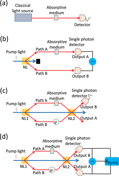
Figure 1. Schematics of the four absorption measurement schemes: CAM (a), QAM (b), LTQAM (c), and HybQAM (d). The phase ϕ in (c) and (d) between the pump light and the photon pairs is tuned to a value where the photon pairs destructively interfere after NL2. NL: nonlinear optical material. The symbol ⊖ in (b) and (d) denotes taking the difference of the photon counts.
Download figure:
Standard image High-resolution image2.2. Quantum-enhanced absorption measurement
To exceed the SNL, a quantum enhanced absorption measurement (QAM) has been proposed and demonstrated [10–15]. Figure 1(b) shows the schematic of a QAM. Pump laser light is injected into a nonlinear optical material (NL) and pairs of photons are generated via a nonlinear optical process, such as spontaneous parametric down-conversion or spontaneous four-wave mixing. The absorptive medium is placed in one of the paths (path A). Each photon is detected by a single-photon detector at the output. Similar to a CAM, we introduce experimental imperfections: the transmittances of the paths A and B (ηA, ηB) and the detection efficiencies of the photon detectors. For simplicity, we assume that the two single-photon detectors have the same detection efficiency ηD. Note that the transmittance of path A (ηA) does not include that of the absorptive medium (T). The initial quantum state of the photon pair emitted from NL is approximately described by

in the low-gain regime where the average photon-pair number per mode α1 is much less than 1 (α1 ≪ 1).  and
and  are the creation operators for A and B modes just after the NL, respectively. Before reaching the single-photon detector, one of the photons in the pair passes through the absorptive medium in path A, while the other photon travels through path B. The creation operators are connected by the relations
where a† and b† are the creation operators for the photons detected at the output A and B, respectively, and  and
and  correspond to the loss. Consequently, the photon-pair state changes as follows:
where  (
( ) and
) and  (
( ) represent the states which have one (zero) photon in the loss modes corresponding to
  and
and  , respectively. In a QAM, the output event number for k trials is given by the count difference between the two single-photon detectors:

with a given number of pairs n = kα1 created from the photon pair source. This means that n is equal to the number of photons input to the optical path where the absorptive medium is placed. The noise in the measurement is determined by the variance of ΔNQAM:
where the last expression is an approximation when α1 ≪ 1. The smallest detectable absorptivity change is obtained from equations (1), (7) and (8).

From equation (2) together with δTQAM, the sensitivity for a QAM is given as follows:

In an ideal case (ηA = ηB = ηD = 1), SQAM becomes  , indicating that the sensitivity to absorption for a QAM increases with T and diverges to infinity at T = 1. This means that the sensitivity for a QAM becomes larger for smaller absorptivity. In other words, a QAM is suited for samples with small absorptivity. In fact, when T ≈ 1, a QAM in the ideal case reaches the quantum Fisher information that determines the smallest uncertainty [32]. However, the performance of a QAM will be significantly degraded due to unwanted photon losses. Since it may be difficult to achieve ηD ≈ 1, while it is relatively easy to improve ηA and ηB closer to 1, let us consider a case where ηD < 1, ηA = ηB = 1 and the sample has a small absorptivity (T ≈ 1). In this case, equation (10) becomes
  . From this, the condition where the SNL is exceeded (SQAM > 1) is given as ηD > 2/3 (figure 2). Therefore, a QAM requires ηD = 66.7% to reach the SNL. Additionally, even with a very high detection efficiency, the enhancement is moderate. For instance, to achieve SQAM = 3, a QAM requires ηD = 94.7%, which is barely reachable using current state of the art photon detectors [33]. SQAM for ηA = ηB ∼ 1 is plotted as a blue curve in figure 2.
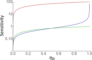
Figure 2. Sensitivity to absorption while changing ηD when ηA = ηB = 1 × 10⁻⁴. The red curve indicates the sensitivity of an LTQAM with γ = 1.0. The blue and green curves indicate the sensitivities of a QAM and a CAM, respectively. The two single-photon detectors for the QAM are assumed to have the same detection efficiency.
Download figure:
Standard image High-resolution image2.3. Loss-tolerant quantum absorption measurement
To suppress the performance degradation due to photon loss at the detection stage in a QAM, we propose a loss-tolerant quantum absorption measurement (LTQAM). Figure 1(c) shows a schematic of an LTQAM. Pairs of photons are generated by a nonlinear optical process in the same way as in a QAM. Then, pump light and the generated photon pairs are injected to the second nonlinear optical material (NL2). The probability amplitude for a photon pair from NL1 interferes with that from NL2. The phase ϕ between the pump light and the photon pairs is tuned to be at the destructive interference condition where the photon pairs vanish. Consequently, when there is no absorptive medium, no photons are found at the output in the condition in which the quantum destructive interference is perfect and there are no optical losses in paths A and B. When the absorptive medium is placed in path A and absorbs one of the photons in a pair, destructive interference does not occur and the other photon will be detected at the output mode. Thus, the photon counts at output B increase with the number of the absorbed photons in the absorptive medium and an absorptivity change is thus detected.
Next, we derive the sensitivity to absorption for an LTQAM. A pair of photons generated from NL1 is represented by equation (5). Since it undergoes a phase-shift ϕ in path B together with losses in paths A and B, as shown in figure 1(c), the quantum state just before NL2 is given by
Then, the pair of photons is injected into NL2 with the pump laser light. After NL2, the photon pair state emitted from NL2 is coherently added to that from NL1 (equation (11)) as follows [18]:
where α0 and α0' are introduced to represent the probability amplitudes of the first two terms which have no photons in the both modes A and B, and α2 is the average number of photon pairs generated from NL2. The mode matching parameter γ determines the ratio of the photon pairs generated from NL2 in the modes A' and B', which do not contribute to the quantum interference but photons in these modes are also detected by the detectors at the outputs. Consequently, γ represents the quality of the interference.
For quantum destructive interference (ϕ = π), equation (12) becomes
The optimal condition for destructive interference is α2 = α1ηAηBTγ, which minimizes the sum of the possibilities of the last two terms in equation (13). This condition is achievable by tuning the power of the pump laser light incident on NL2. In determining α2, we can obtain α1, ηA, ηB and γ by independent measurements in advance. Although the exact value of T is unknown in advance, T can be approximately set to be 1 for measuring very small absorptivity, and thus it is possible to substantially determine α2. After optimizing α2, we obtain the following state:
Considering the photon losses at the photon detectors, this quantum state changes as follows:
where  ,
,  and
and  are introduced to represent the probability amplitudes of the terms which have no photons in the both modes A and B, and
  (
( ) and
) and  (
( ) represent the states which have one (zero) photon in the loss modes of the output A and B, respectively. In an LTQAM, we measure the number of photons at the output B. For k trials, the average number of detected photons is given by
where pB is the probability that a photon is detected at output B and b' and b'† are the annihilation and creation operators for mode B'. The noise in this measurement is given by  and the smallest detectable absorptivity change is obtained from equations (1) and (16) as
where the second equation is approximated to the last under the assumption α1 ≪ 1. From equations (2) and (17), the sensitivity to absorption for an LTQAM is


In the simplest case where ηA = ηB = γ = 1 and ηD < 1, SLTQAM is always higher than SQAM because  and
and  , demonstrating the loss-tolerance of an LTQAM. In the situation of interest, the absorption is so small that T ≈ 1. In this case, SLTQAM can be much higher than 1 even when the QAM is inferior to the SNL (SQAM < 1).
Figure 2 shows the sensitivities while changing ηD when the transmittances of the paths A and B are ηA = ηB = 1 × 10⁻⁴, which is achievable with current state of the art technology [34]. We assume that the absorptive medium has a very small absorptivity of 10−6 (namely T = 1 × 10⁻⁶). Note that this value itself is unimportant in the following analysis because the condition 1 − T ≪ 1 − ηA is satisfied, and in this case, the change in T negligibly affects the sensitivity. The red curve in figure 2 shows the sensitivity for an LTQAM when the quantum destructive interference is perfect (γ = 1). While the sensitivity to absorption for a QAM (blue curve in figure 2) rapidly decreases with ηD and is lower than that for a CAM (green curve in figure 2) with ηD below 0.5, an LTQAM maintains an advantage even for lower ηD.
In figures 3(a) and (b), we show the sensitivity to absorption when ηA and ηB are varied, respectively, while ηB and ηA are fixed to 1 × 10⁻⁴ in order to check how ηA and ηB affect the sensitivity to absorption. We adopt a detection efficiency ηD of 0.80, which is achievable with commercial single-photon detectors. The two single-photon detectors in the LTQAM and QAM are assumed to have the same detection efficiency. Because the sensitivity for an LTQAM diverges to infinity at ηA = 1.0 when γ = 1.0, we set the plot range for ηA to be from 0 to 1 × 10⁻⁴ in figure 3(a). A comparison of figures 3(a) and (b) reveals that the sensitivities for an LTQAM have a stronger dependence on ηA than on ηB, and thus increasing ηA is more effective for improving the sensitivity. In figure 3(a), the LTQAM is inferior to the CAM for ηA less than around 0.5. This can be explained by equation (19), which indicates that ηA affects the sensitivity SLTQAM in exactly the same way as γ.
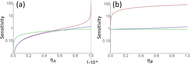
Figure 3. Sensitivity to absorption while changing the path transmittances ηA (a) and ηB (b). The detection efficiency is fixed at ηD = 0.80. The red curve indicates the sensitivity of an LTQAM with γ = 1.0. The blue and green curves indicate the sensitivities of a QAM and a CAM, respectively. The two single-photon detectors for the QAM are assumed to have the same detection efficiency (ηD = 0.80). The sensitivity for the CAM does not depend on ηB because the path B does not exist in the model of the CAM.
Download figure:
Standard image High-resolution imageTo analyze the effect of imperfection in the destructive quantum interference, figure 4 shows the sensitivities while changing the mode matching parameter γ when ηA = ηB = 1 × 10⁻⁴. The detection efficiency ηD is set to 0.80 and 0.67 for figures 4(a) and (b), respectively. The sensitivity to absorption for an LTQAM (red curve in figures 4(a) and (b)) rapidly decreases with γ. When ηD = 0.80, the thresholds of γ where an LTQAM surpasses a QAM (blue curve in figure 4(a)) and a CAM (green curve in figure 4(a)) are 0.77 and 0.62, respectively. Figure 4(b) shows the case for ηD = 0.67 where the sensitivity to absorption for a QAM is equal to the SNL (SQAM = 1). In this case, while a QAM does not show a quantum advantage, an LTQAM can exceed the SNL for γ larger than 0.69.
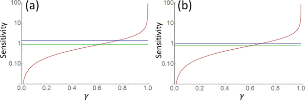
Figure 4. Sensitivity to absorption while changing γ for ηD = 0.80 (a) and ηD = 0.67 (b). The path transmittances are set to ηA = ηB = 1 × 10⁻⁴. The red curve indicates the sensitivity for an LTQAM. The blue and green curves indicate the sensitivities for a QAM and a CAM, respectively. The two single-photon detectors for the QAM are assumed to have the same detection efficiency.
Download figure:
Standard image High-resolution image2.4. Hybrid QAM
In LTQAM, photons are not found at output A when there is no experimental imperfection. However, if the quantum destructive interference is imperfect and/or the transmittance of path B is not unity, photons leak to output A. In this case, the information about absorptivity which the leaked photons have is discarded because the leaked photons are not detected in an LTQAM. To solve this problem, we also propose a hybrid approach (HybQAM) in which an additional single-photon detector at output A detects the leaked photons, as shown in figure 1(d).
Next, we derive the sensitivity to absorption for HybQAM. We consider a linear combination of the detected photon counts as follows:

where NA and NB are the detected photon counts at the output A and B, respectively, and m and l are the weights of NA and NB, respectively. From equations (15) and (20), NHybQ becomes

The noise of the measurement ΔNHybQ is obtained in a similar way to equation (8). The smallest detectable absorptivity change is derived as follows:

which is approximated using the assumption α1 ≪ 1. From the definition of the sensitivity shown in equation (2), the sensitivity of HybQAM is given by

SHybQ will be maximized when m and l satisfy the following relations:


MATHEMATICA was used to find this condition. For an extreme example where γ = 0 and ηA = ηB = 1,  , whereas SLTQAM = 0, which shows that the HybQAM is resistant to decreasing γ. Note that in an ideal case for LTQAM where ηA = ηB = γ = 1, SHybQ becomes the same as SLTQAM:
  .
.
Figure 5 shows the sensitivity to absorption while changing γ. As for figure 4, the detection efficiency ηD is set to be 0.80 and 0.67 for figureS 5(a) and (b), respectively. The other parameters ηA and ηB are set to be the same as those used in figure 4, namely 1 × 10⁻⁴. The red curve indicates the sensitivity for HybQAM. Compared with the LTQAM shown in figure 4 (red curve), the HybQAM maintains a sensitivity higher than both the QAM (blue curve) and the CAM (green curve) for any γ. Figure 5(b) shows the case for ηD = 0.67 where the sensitivity to absorption for the QAM is equal to the SNL (SQAM = 1). We can see that the HybQAM exceeds the SNL for all γ even when the QAM does not show a quantum advantage.

Figure 5. Sensitivity to absorption while changing γ when ηA = ηB = 1 × 10⁻⁴, ηD = 0.80 (a) and ηD = 0.67 (b). The red curve indicates the sensitivity for the HybQAM. The blue curve and green curve indicate the sensitivities for the QAM and the CAM, respectively. The two single-photon detectors for the QAM and HybQAM are assumed to have the same detection efficiency.
Download figure:
Standard image High-resolution image
The above results show that improving γ is important for achieving a high sensitivity for both LTQAM and HybQAM. Although there have been no reported values of γ, it is possible to estimate it from the fringe visibility of a nonlinear interferometer. For instance, from the fringe visibility of 0.965 reported in reference [35], we can obtain a lower bound of γ of 0.931. Note that γ for this experiment would be higher when the loss in the setup is compensated. We believe that the recent intensive investigations of nonlinear interferometers will meant that nearly perfect mode-matching in nonlinear interferometer can be achieved in the near future.
3. Conclusion
In conclusion, we have proposed a LTQAM using quantum destructive interference. Our theoretical results show that our scheme surpasses the conventional quantum scheme (QAM) under photon loss at the detection stage. The performance of a QAM is rapidly degraded with photon loss at the detection stage (ηD). Even without photon loss in the optical paths (ηA = ηB ∼ 1), a QAM requires ηD > 0.67 to exceed the SNL, and ηD > 0.96 to achieve a sensitivity of three times the SNL. In contrast, the sensitivity of an LTQAM is higher than the SNL at almost all ηD for ideal quantum interference (γ = 1) and it can achieve a sensitivity of more than 30 times the SNL even when ηD = 0.1. To cope with the case where the quantum interference is experimentally limited (γ < 1), we have also proposed a hybrid approach (HybQAM). We found that a HybQAM outperforms a QAM even for a limited quantum interference (γ < 1). Even when a QAM does not show a quantum advantage due to a low ηD, a HybQAM can exceed the SNL for any γ. We believe that our results are promising for achieving a quantum advantage in imaging and absorption spectroscopy of an object with very small absorptivity, such as single molecules.
Acknowledgments
The authors wish to thank Prof. Masazumi Fujiwara for helpful discussions. This work was supported in part by JST-PRESTO (JPMJPR15P4), a Grant-in-Aid from JSPS (17H02936, 25620001, 25707034, 18K18733, 26220712) and JST-CREST (JPMJCR1674).