


Abstract
The well-known schemes (e.g. Brunel mechanism, resonance absorption,  heating etc) couple laser energy to the lighter electron species of the plasma. In this work, a fundamentally new mechanism of laser energy absorption directly to the heavier ion species has been proposed. The mechanism relies on the difference between the
  drifts of electron and ions in the oscillating electric field of the laser and an external magnetic field to create charge density perturbations. The proposed mechanism is verified with the help of particle-in-cell (PIC) simulations using OSIRIS4.0.
Export citation and abstract BibTeX RIS

Original content from this work may be used under the terms of the Creative Commons Attribution 4.0 licence. Any further distribution of this work must maintain attribution to the author(s) and the title of the work, journal citation and DOI.
1. Introduction
There are many well-known schemes by which the laser energy can get absorbed in the plasmas [1, 2]. For instance, resonance absorption, Brunel,  heating schemes etc [3–9]. All these schemes rely on the dynamical response of the lighter electron species in the presence of the oscillating field of a high frequency laser. Consequently, the dominant transfer of energy from laser occurs in electron species. However, there are many applications (e.g. fast ignition of fusion targets [10–12], cancer radiotherapy [13], proton radiography [14, 15], production of warm dense matter [16] etc) where it is desirable to have energetic ions. This has led to efforts seeking efficient mechanisms of ion heating and/or acceleration [17–21]. In many previous studies, a two step approach has been envisaged for this particular objective. The laser energy is first absorbed by electrons and its transfer to ions depends on the electron–ion classical collisional and/or anomalous processes. Since Rutherford's collision cross section decreases with increasing electron energy, this process is inefficient at high energies [22]. Many ideas of anomalous transfer of energy from electron to ion have also been proposed [23–30]. There have been studies where indirect ways of coupling laser energy into ions via ponderomotive force [31, 32] and formation of collisionless shock [33] have been shown. In this work, we propose a novel scheme by which direct transfer of laser energy to ions is possible.
The new mechanism relies on the application of a strong external magnetic field normal to the laser propagation and also the polarization direction. Strength of the magnetic field is chosen such that it restricts the motion of electrons which are tied to the magnetic field lines but the heavier ion species remain un-magnetized and are relatively free to move in response to the laser electric field. This happens when the electron gyroradius is smaller than the laser wavelength whereas ion gyroradius is larger compared to it, as depicted in the schematic of figure 1. The frequency condition ωce > ωl > ωci needs to be satisfied. This requirement demands that the applied external magnetic field strength B0 should be greater than mecωl/e.

Figure 1. Schematic (not to scale) showing that under the condition ωce > ωl > ωci, the electrons are tightly bound to the external magnetic field (along  ) whereas ions are free to move under the effect of laser. The direction of oscillating electric field due to laser is along
  and that of laser magnetic field along with a static external magnetic field is along and the laser propagation is along
  direction.
  drift due to oscillating electric field is acting along
  .
.
Download figure:
Standard image High-resolution imageThe  drift velocity in the presence of an externally applied magnetic field and an oscillating electric field is given by

as ωce > ωl > ωci, the drift velocity of the two species differ [34]. Here, the suffix s = e, i represents the electron and ion species respectively. Thus, ωce and ωci stands for the electron and ion cyclotron frequency respectively. Furthermore, ωl stands for the laser frequency. As mentioned earlier the magnetic fieldis chosen so that the condition ωce > ωl > ωci is satisfied. This ensures that the electrons motion is predominantly governed by  drift given by equation (1). Ions, on the other hand, being un-magnetized are essentially accelerated by the electric field acting on them. Magnetic field has negligible role on them.
The difference in the drift velocities of electrons and ions gives rise to a current. Since, the laser electric field and the externally applied magnetic field, both are perpendicular to the propagation direction, the electrons drift produces current along the laser propagation direction. This current has a spatial variations at the laser wavelength due to its dependence on the electric field of the applied laser. This spatial variation leads to a finite divergence of the current which drives a charge density fluctuation given by the continuity equation:

This generates electrostatic plasma mode in the system, thereby, the energy of the laser gets transferred to plasma. This is the underlying main principle on which our new mechanism has been proposed. It should be noted when the applied magnetic field is zero,  (as ωcs = 0) for both the species, and no charge separation will be created in the plasma. In the other limit of a very large magnetic field, both ions and electrons are magnetized and move with identical drift velocity
  following equation (1). Thus in this limit also one should expect no charge density fluctuation. Thus, in both the limits the proposed mechanism of laser energy absorption will be inoperative. We have carried out PIC (particle-in-cell) simulations through OSIRIS-4.0 to support this mechanism.
As pointed out earlier, the experimental implementation of this mechanism requires an application of an external magnetic field of magnitude B0 > meωlc/e. For a typical laser of 1 μm wavelength this translates to a requirement of magnetic field of the order of 104 Tesla. The CO2 lasers which have a 10 μm wavelength, reduces the requirement by ten times. Lately, there has been a rapid technological progress in achievinghigh magnetic field in the laboratory [35, 36]. The value of 1.2 kilo Tesla [37] at Institute for Solid State Physics at the University of Tokyo, Japan has already been achieved. Thus, it is only a matter of time before the requirement for carrying out experiments in this domain would be possible.
2. Simulation details
We use OSIRIS-4.0 framework [38–40] for our particle-in-cell (PIC) studies. The schematic (not to scale) in figure 1 shows the field configuration used in the simulation. The  is the propagation direction of the laser. The laser electric field is along and the applied external magnetic field is along as shown in the figure. A 2D rectangular simulation box with dimensions Lx = 3000c/ωpe and Ly = 100c/ωpe has been chosen. The number of particles per cell are taken to be 4. The plasma boundary starts from x = 500c/ωpe onward. There is vacuum between x = 0 to x = 500c/ωpe. The spatial resolution is taken as 10 cells per electron skin depth corresponding to a grid size Δx = 0.1c/ωpe and time step for calculations is taken tobe
  . There is a sharp plasma–vacuum interface and laser is incident from left side on the plasma target. We consider a p-polarized, plane short-pulse laser of wavelength λl = 9.42 μm corresponding to CO2 laser. The choice of long-wavelength laser is simply for the sake of definiteness and is motivated by the fact that it reduces the requirement of the externally applied magnetic field. The mechanism, however, is independent of the laser wavelength. The normally incident laser is propagating along
  , centred at x = 250c/ωpe and has a pulse length ranging from x = 0 to 500c/ωpe. The peak intensity of laser is taken to be I = 3.5 × 10¹⁵ W cm−2 with a Gaussian profile having rise and fall time of
  each. The laser is taken to be infinite in transverse direction in most of the runs. This is chosen purposefully to avoid edge effects which might interfere with the effects arising from
  which we wish to clearly identify. We have, however, also carried out a few simulation with laser pulse having finite transverse extent. The characteristics features do not differ significantly for the two runs. Boundary conditions for fields and particle are periodic in transverse direction and absorbing in longitudinal direction. The number density of the plasma is taken to be n0 = 3 × 1020 cm−3 for which the electron plasma frequency is equal to 1015 rad s−1. Hence the plasma is overdense for the incident laser pulse.
We have followed the dynamics of both electrons and ion species. The simulations are, however, carried out at a reduced mass of ions which is taken to be 25 times heavier than electrons (i.e. mi = 25me, where mi and me denote the rest mass of the ion and electron species respectively). This mass ratio has been chosen to reduce the computational time. We use normalised units henceforth, unless otherwise stated explicitly. The time is normalised by the inverse of electron plasma frequency corresponding to the chosen plasma density of n0. The laser frequency is chosen to be ωl = 0.2ωpe, which is smaller than the electron plasma frequency but matches with the ion plasma frequency ωpi with mass ratio of mi/me = 25 chosen here. This choice has been made to observe the possible resonant excitation of ion mode. We have, however, also carried out simulations with laser frequencies of ωl = 0.15ωpe and ωl = 0.12ωpe which differ from the ion plasma frequency. The length is normalised by electron skin depth c/ωpe and the magnetic field by mecωpe/e. The external magnetic field has been chosen in such a way that ωce > ωl > ωci. To satisfy this condition the value of magnetic field is chosen to be B0 = 2.5 mecωpee−1. For this field, the electrons gyrate at a frequency 2.5ωpe. The simulation geometry is specifically chosen to avoid the possibility of any well-known absorption schemes to be operative. The laser is incident normal to the sharp plasma interface. This ensures the absence of resonance and vacuum heating schemes. Also, the role of  electron heating is made negligible by choosing the laser intensity to lie in the non-relativistic domain of a0 = eE/meωlc < 1 (a0 = 0.5 corresponding to CO2 laser). The simulation values of various laser and plasma parameters in both normalised and standard units have been provided in table 1.
Table 1. A comparison of normalised and possible experimental values of simulation parameters.
| Parameters | Normalised units | Possible values in standard unit |
|---|---|---|
| Laser parameters | ||
| Frequency | 0.2 | 0.2 × 10¹⁵ Hz |
| Wavelength | 31.4 | 9.42 μm |
| Intensity | a0 = 0.5 | 3.5 × 10¹⁵ Wcm−2 |
| Plasma parameters | ||
| Number density | 1 | 3 × 1020 cm−3 |
| Electron plasma frequency | 1 | 1015 Hz |
| Ion plasma frequency | 0.2 | 0.2 × 10¹⁵ Hz |
| External magnetic field parameters | ||
| B0 | 2.5 | 14.14 kT |
3. Observations and discussions
We first provide a comparison between two cases, namely (A) for which the applied magnetic fieldB0 = 0 and (B) for which B0 = 2.5. The choice of B0 = 2.5 ensures that the condition ωce > ωl > ωci is satisfied. For these simulations there is no transverse variation of the laser pulse and hence the simulation configuration is symmetric in the y coordinate, we choose to depict the fields as a function of the coordinate x in the figures.
In figure 2, the three subplots in the first row depict the plot of the time-dependent magnetic field associated with the laser and the self-consistent response of the plasma medium as a function of x at three distinct time (i) t = 0 showing the initial laser pulse field when it does not touch the plasma surface, (ii) t = 350 when the laser has touched the plasma and (iii) t = 700 when the laser pulse has been reflected from the plasma surface and the plasma is left with the remnant self-consistent excitations. The dashed red line denotes the case (A) for which B0 = 0 and the solid blue line corresponds to case (B) with B0 = 2.5.It can be observed from the figure that in case (A) there is no penetration of the laser magnetic field in the plasma and almost a complete reflection of the pulse occurs. However, for case (B) when the external applied field B0 is finite and equal to 2.5, a part of the laser field shows clear penetration in the plasma medium. In the same figure the second row of three subplots show the plasma current Jx as a function of x for the two cases. Third and last row depicts the electrostatic field Ex generated in the plasma medium. It is evident from the plots of Jx and Ex that while the plasma gets stirred significantly by the laser field in the presence of applied external magnetic field in case (B), for case (A) the plasma continues to remain quiescent even after interacting with the laser pulse. This is as expected by our proposed mechanism.

Figure 2. Time evolution of spatial variation of Bz (normalised to mecωpe/e), x-component of total current Jx (normalised to n0ec) and x-component of electric field Ex (normalised to mecωpe/e) with respect to  , averaged over , showing that as laser interacts with plasma (t = 350), there is a finite magnitude of perturbed Bz, Jx and Ex in case (B) (with external magnetic field) which is absent in case (A) (without external magnetic field). From these plots, we can infer that a part of laser energy has been coupled into plasma.
Download figure:
Standard image High-resolution imageWe now compare the evolution of various energies for the two cases in figure 3. We indicate distinct time incidents by vertical lines in this figure. The first two solid black lines denote the times t1 = 100and t2 = 380, where t2 − t1 region indicates the time interval during which the laser interacts with the plasma. Thereafter, laser field gets reflected from the plasma surface. At around t3 = 500 denoted by the black dashed line, the laser reflects from the plasma surface and at t4 = 780 indicated by black dotted line the laser field leaves the simulation box. Evolution of the electromagnetic field energy has been shown by the blue dashed and solid lines for case (A) and case (B) respectively. The left side of the y-axis in the figure represents scale for this particular energy. The electromagnetic field energy remains constant associated with the laser pulse till t1. At t1 the laser pulse interacts with the plasma surface. There is a fall of electromagnetic energy from t1 to t2, the time for which the laser pulse interacts with the plasma medium.It is evident from figure that the electromagnetic energy decreases more in case (B) than in case (A) during this period. From t2 to t3 the laser pulse reflects from the plasma surface but remains within simulation box therefore, the electromagnetic energy remains constant. At t3 the left edge of the reflected laser pulse touches the left boundary of the simulation box. Thereafter there is a continuous decay in the field energy till t4 at which the pulse completely leaves the simulation box. Thus, while the first fall of the electromagnetic field energy between t1 to t2 is associated with the laser pulse interacting with the plasma medium, the second fall of the electromagnetic energy between t3 to t4 is due to the laser pulse leaving the simulation box. The laser energy transfer, therefore, essentially occurs between t1 to t2. Further, it should be noted that the energy transfer to plasma medium is more in case (B) with externally applied magnetic field. Clearly, this energy transfer to plasma would be in the form of field and kinetic energies. Another interesting thing to observe is that even after the laser pulse leaves the system, electromagnetic energy for case (B) remains finite in contrast to case (A) where it falls off to zero. This shows that the laserinteraction creates some electromagnetic field fluctuation in the plasma medium in case (B).

Figure 3. Time variation of mean electromagnetic field (Emf) energy density of the system (left y axis) and kinetic energy density of both the species (right y axis) showing that laser energy is mainly gained by electrons in case (A) (B0 = 0) and by ions in case (B) (B0 = 2.5). The decrease in Emf energy of the system between the two solid lines is due to the interaction of laser with plasma (there is gain in kinetic energy of electrons in case (A) and ions in case (B) at the same time). Between dashed and dotted line, the laser reflects back and moves out of the simulation box and as a result, we observe a drop in Emf energy of the system. There is also generation of some electrostatic mode in plasma in case (B) contributing to Emf energy of the system even after the laser has been reflected out of the simulation box (beyond dotted line). The total energy of the system is shown by purple lines for both the cases. Total energy is constant till laser is in the simulation box and begins to fall as the laser starts leaving the simulation box.
Download figure:
Standard image High-resolution imageThe evolution of kinetic energy of electrons and ions are shown by green and red color line plots respectively in the same figure 3. The dashed and dotted lines are for case (A) and the solid line with dots correspond to case (B). For these kinetic energy plots, the right y-axis defines the scale. In absence of applied magnetic field in case (A) the gain in ion energy is much smaller compared to that of electrons. However, for case (B) in the presence of magnetic field the kinetic energy of ions is much higher than that of electrons. The total energy absorbed by plasma in this case is also higher.
One can infer that the laser interacts with plasma in case (B) in a more efficient fashion and excites certain disturbances in the plasma. Disturbances that are excited in case (B) do have an electrostatic characteristic as evident from the evolution of the x component of the electric field Ex shown in figure 4(a) at location x = 540c/ωpe (which is deep in the bulk region of the plasma medium). For case (A) the amplitude of the electrostatic field Ex is negligible. The frequency associated with the regular oscillation in the electric field Ex is identified by carrying a Fourier transformation which is shown in figure 4(b). We take the Fourier transform of self generated electric field (Ex) in bulk plasma (at x = 540) after laser hasreflected back from the plasma boundary. The peak in Fourier transform for the two cases appear at very distinct frequencies. In case (A) the spectrum shows a peak at ω = 1 which is the electron plasma frequency. On the other hand, for case (B) the peak in the frequency is shifted at a lower side (corresponds to a value close to ∼0.2) which is indicative of an ion dominated mode, the ion plasma frequency being 0.2. The peak frequency is found to be dependent on externally applied magnetic field which suggests the presence of lower hybrid mode. We have also carried out simulations with a few other values of laser frequencies for example ωl = 0.15, 0.12 in addition to 0.2. The FFT for all these cases have been compared in figure 5 and it can be observed that despite differences in the laser frequency the electrostatic mode that is excited has the same frequency.

Figure 4. (a) Time variation of x-component of electric field Ex for both the cases at x = 540 c/ωpe, averaged over , showing generation of electrostatic mode in the bulk plasma in case (A) (B0 = 0) and case (B) (B0 = 2.5). (b) Fast Fourier transform of Ex showing peak at electron plasma oscillation for case (A) and at a lower frequency for case (B). The shift in the frequency towards lower end in case (B) indicates presence of an ion dominated mode.
Download figure:
Standard image High-resolution image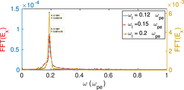
Figure 5. FFT of self generated electric field component Ex in bulk plasma (at x = 540) for three different values of laser frequencies after laser has been reflected back. Left y-axis is for ωl = 0.12ωpe and ωl = 0.15ωpe and right is for ωl = 0.2ωpe.
Download figure:
Standard image High-resolution imageThe oscillations in electrostatic field are a result of space charge fluctuations excited in the plasma.The number density and the velocity fluctuations associated with the two species have been shown in the first and second row of the figure for the two species of electron and ions by blue and red colour lines respectively as a function of  at three different times (figure 6). The third row of subplots shows the current density fluctuations. It is clear from the plot that except for the short distance near the plasma boundary at x = 500, the ion and electron density oscillations and their x component of the velocities are in tandem. These oscillations propagate deeper in the plasma with time. The laser interacting at the plasma boundary excites a space charge fluctuations at the boundary which then travels in the bulk region of the plasma.
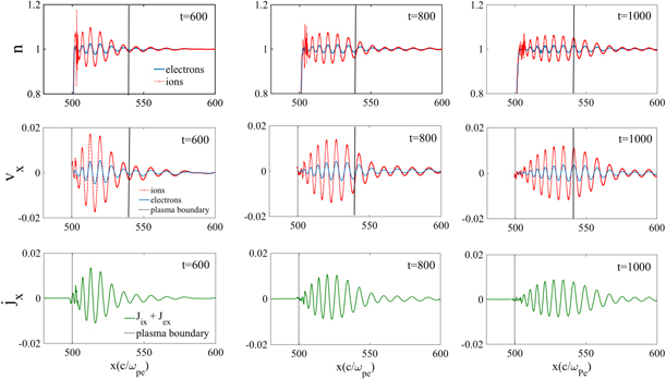
Figure 6. Figure shows the spatial variation of density (n), x-component of velocity, Vx and x-component of total current, Jx averaged over at different times [for case (B), B0 = 2.5]. At a particular time we observe that the density perturbations created and the difference in drift velocity of both the species (Vix − Vex) are at the same position, indicating the correspondence between them. Solid line in the plots of n and Vx correspond to x = 540 which is the chosen spatial location in figures 8 and 11.
Download figure:
Standard image High-resolution imageWe now compare the theoretical value of the velocity as expected from the mechanism put forward by us with that obtained from simulation for both the species (figure 7). It can be observed from the figure that the electron velocity is pretty low compared to the ion velocity. The electrons are magnetized and the x component of its velocity follow the theoretical expression of equation (1). It can be observed (from the left subplot of figure 7) that there is a good agreement between the theoretical expression and the value obtained in the simulation. The heavier ion species is un-magnetized as per our choice of magnetic field value and hence its dominant velocity along x is ultimately provided by the direct acceleration due to the x component of electric field vector Ex which gets created self consistently by the space charge separation. The close match between theoretical and simulation are in confirmation with our proposed scheme.
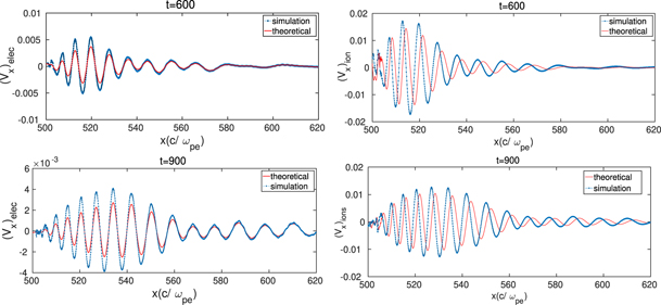
Figure 7. A comparison of the theoretical and simulation value of Vx for electrons and ions at different times. In the theoretical curve for electrons, we plot Vx given by equation (1). In the theoretical curve for ions, we plot Vx = eEx/mω.
Download figure:
Standard image High-resolution imageIn figure 8 we show a plot of the velocity and density fluctuations of the two species as a function of time for x = 540 (a point in the bulk region of the plasma). The plots correspond to six different values of the magnetic field. From the plots it is clear that at low values of the magnetic field velocity fluctuations are small. At an intermediate value of the magnetic field B0 = 2, 2.5, 3.0 the velocity fluctuations increase and the difference between electron and ion velocity is also high. The number density fluctuations are also high for these cases. However, at very high value of magnetic field of B = 10 the electron and ion velocities are almost similar and the number density fluctuation is small. It should be noted that at the intermediate value of B = 2, 2.5, 3.0 only the required condition of ωce > ωl > ωci is satisfied. For B = 10, the ions too get magnetized. This is consistent with our proposed mechanism in which the number density fluctuation are supposed to be excited by the difference in the  velocity of the two species. The difference in drift velocity of the two species vanishes in both the limits of low and high magnetic fields. This is yet another confirmation of the proposed mechanism.

Figure 8. Figure showing the effect of varying external magnetic field on Vx(t) and density perturbations of both the charged species at a particular value of  (here, x = 540), averaged over (for case (B), B0 = 2.5). With increasing applied magnetic field, difference in velocity of both the species (Vix − Vex) increases, when ωce > ωl > ωci is satisfied. As soon as ωce > ωl > ωci is not satisfied (B0 = 10), Vix − Vex again decreases. Similar trend is observed in density perturbations of both the species as well.
Download figure:
Standard image High-resolution imageThese number density fluctuations associated with ion time scale of response peak at an intermediate value of B0 (the applied magnetic field). The mode disappears both at the low magnetic field and also at the higher values of the magnetic field. To understand the role of magnetic field on laser absorption, we show in table 2 the total energy absorbed by the two species (electrons and ions) from the laser for various values of the applied magnetic field. From this table, it is clear that the energy absorption in ions is low both at the low value of magnetic field and also at the high value of the magnetic field. This has also been depicted in the plot of figure 9 showing the total energy absorption by electrons and ions at various values of the external magnetic field. We have also shown variation of x-component of total current, Jx with applied magnetic field and observe that ion absorption follows the profile of Jx as a function of the applied magnetic field. Here the values are to be taken as indicative of the qualitative trend. The quantitative values will differ if real mass ratio of the two species are chosen.
Table 2. Laser energy absorbed by ions increases as applied external magnetic field increases. It can also be noted that the ion energy is significant for the case only when Vix − Vex is finite (figure 8) which is only true if ωce > ωl > ωci is satisfied. The table is indicative of qualitative trend. The quantitative values will differ for real mass ratio. The numbers alongside in brackets corresponding to B = 2.5, show % of laser energy absorbed for the case of simulations performed for a finite transverse extent of laser pulse.
| Externally applied magnetic | % of laser energy | % of laser energy | % of laser energy |
|---|---|---|---|
| field (in normalised units) | absorbed by electrons | absorbed by ions | absorbed by plasma |
| Bz = 0 | 6.06 | 2.40 | 8.46 |
| Bz = 1.5 | 0.42 | 2.76 | 3.18 |
| Bz = 2 | 0.42 | 9.68 | 10.10 |
| Bz = 2.5 | 0.58 (0.77) | 14.52 (13.74) | 15.10 (14.51) |
| Bz = 3 | 1.22 | 31.12 | 32.34 |
| Bz = 3.5 | 1.41 | 44.60 | 46.01 |
| Bz = 4 | 0.22 | 10.98 | 11.2 |
| Bz = 5 | 0.003 | 0.61 | 0.61 |
| Bz = 7 | 0.002 | 0.002 | 0.004 |
| Bz = 10 | 0.002 | 0.005 | 0.007 |
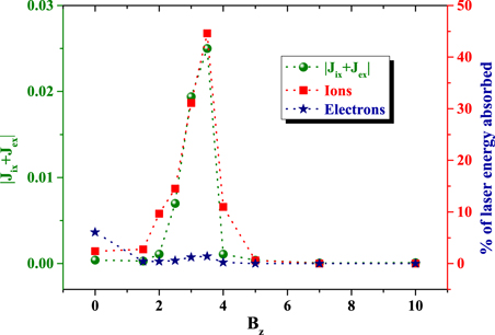
Figure 9. Figure shows the effect of varying external magnetic field on the total current generated in the system (left y axis) and energy absorbed by electrons and ions (right y axis). It can be observed from the graph that the energy absorbed by ions follow the total current in the system. Also, total current as well as energy absorbed by ions increase only when ωce > ωl > ωci.
Download figure:
Standard image High-resolution imageThe particle count of the two species as a function of their acquired kinetic energy has been shown in figure 10 for the two cases (A) and (B). From this figure one can infer clearly that energy absorption by ions in the presence of external magnetic field is higher.
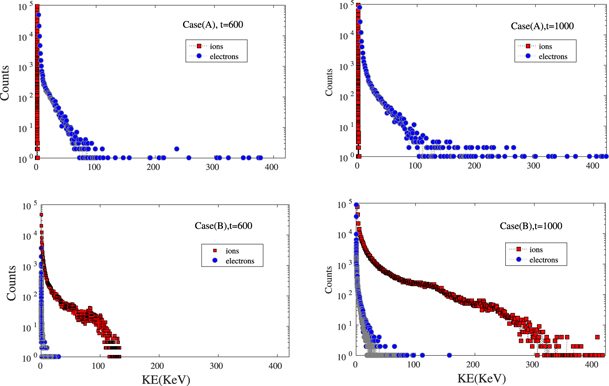
Figure 10. Energy distribution of ions and electrons for case (A) (B0 = 0) and (B) (B0 = 2.5) showing the maximum energy gained by them in both the cases. In case (A), since no external magnetic field is present, therefore laser energy is mainly taken up by electrons whereas in case (B), due to the presence of an external magnetic field such that ωce > ωl > ωci , electrons are magnetized but ions are still unmagntised which imparts more energy to ions in case (B).
Download figure:
Standard image High-resolution imageWe have chosen to show in figure 11 some particle related diagnostics for a set of 10 randomly chosen electrons (represented by blue color) and 10 ions (shown by red color). In subplot (a) their locations have been shown at t = 0 and subplot (b) and (c) show their particle trajectories from initial time to t = 500and t = 998 respectively. Since there are several particles in the frame the details of the trajectory of each particle is not evident from these plots. We have, therefore, added another subplot (d) in the figure where we have chosen to represent the trajectory of one particular set of electron and ion in an expanded x and y scale. From this plot it can be observed that the particles have an oscillatory motion in space. In subplot (e) we plot the x location of two particles (electron and ion) as a function of time which clearly shows the oscillatory motion of ions and electrons. The amplitude of ion oscillation is higher than that of electrons. A small steady drift along the positive x direction for both of them can also be observed initially. This is because for a finite temporal electromagnetic wave pulse it is well known that a charge particle gets displaced along the laser propagation direction. The particles, however, oscillate with increasing amplitude.
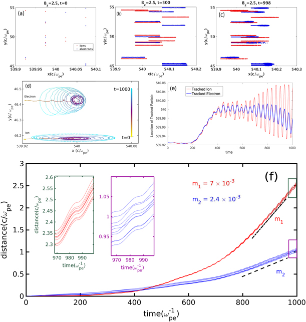
Figure 11. Subplots (a) shows the location of snapshots of 10 particles of both species (blue for electron and red for ion) at t = 0 chosen randomly in the plasma, which have been tracked till t = 500 and t = 998 in subplot (b) and subplot (c) respectively. In subplot (d) we have shown one particular set of electron and ion trajectories in an expanded x and y scale which clearly shows that the particles oscillate with increasing amplitude. In subplot (e) we have plotted the x location of these two particles as a function of time. Clearly, the ions oscillate with higher amplitude. In subplot (f) we have chosen to plot total distance ( . Here i represents the ith time step and Δxi is the displacement of the particle in ith time step) traversed by all the tracked particles along
  till t = 1000. It can be seen that the total distance traversed by ions is more than electrons which indicates that ions have higher average speed than electrons. The typical estimate of the average speeds of ions and electrons is provided by the slopes m1 and m2 respectively. In the inset of this subplot we have shown the expanded view of the selected boxes to demonstrate clearly the plots corresponding to all the chosen particles. It is evident that the particles of same species move with identical average speed.
Download figure:
Standard image High-resolution imageAn estimate of average speed along x for the two species have been provided. In subplot (f) of figure 11 we plot the total distance dx covered in x by the particles whose position and trajectories have been depicted in other subplots (a–c) of figure 11. Here  , where i represents the ith time step and Δxi is the displacement of the particle in ith time step. We have also shown the expanded plot of dx in the inset of this subplot (f) for a clear view. From the slope of the plot of dx with time we have estimated the average speed of ions and electrons which have been listed in the plot as vsi = m1 = 7 × 10⁻³ and vse = m2 = 2.4 × 10⁻³. These values compare well with the average speed that can be estimated from figure 6, in terms of the maximum amplitude and assuming the variation to be sinusoidal. Thus,
  and
and  which compare well with vsi and vse respectively. Here vmi and vme are the observed amplitude of electron and ion velocities shown in figure 6.
We have also carried out simulations with a laser of finite transverse extent to see the importance if any of 2D effects associated with the edge of the laser pulse. The laser pulse is chosen to have Gaussian profile in both  and the transverse direction.
The tranverse FWHM of the laser spot size is 150c/ωpe. Other laser parameters are kept same as before. A rectangular box with dimensions Lx = 2000c/ωpe and Ly = 2500c/ωpe is chosen.
The 2D color plots depicting the case of finite transverse laser beam and the laser with infinite extent has been shown in figure 12. It can be observed that the ion density and current structures are similar in both the cases. The peak frequency in FFT of Ex also points at the same frequency in both cases (figure 13). The fractional count of electrons and ions as a function of acquired energy has been shown in figure 14 for the finite and infinite transverse laser pulse. From this figure it is clear that the energy acquired by ions is higher than that of electrons for both cases. The % of laser absorption for this particular simulation corresponding to Bz = 2.5 has been mentioned in the table 2 in brackets alongside which is similar to that of infinite laser case.

Figure 12. Current density (Jx) as a function of  averaged over superposed over colorplot of charge density of ions. It can be observed that current induced in the system follows the density perturbation of ions. Since the transverse box size is different for both the cases mentioned above, therefore, quantitative comparison between the magnitudes of Jx should not be done.
Download figure:
Standard image High-resolution image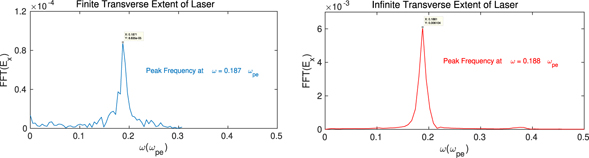
Figure 13. FFT of Ex showing the peak frequency for finite and infinite transverse extent of laser. The peak frequencies are very close to each other in both cases. FFT has been done at a location in bulk plasma (x = 540), averaged over .
Download figure:
Standard image High-resolution image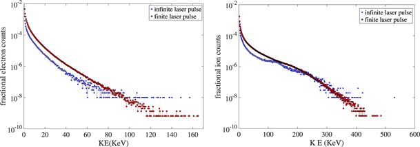
Figure 14. Kinetic energy of electrons and ions for finite and infinite transverse extent of laser pulse at t = 1000. It can be seen that ion energy in both cases is more than electron energy. The area of simulation box is more for the case of finite laser pulse simulation, therefore, number of particles differ for the two cases.
Download figure:
Standard image High-resolution image
4. Conclusion
The results of the previous section clearly demonstrate that the laser energy gets preferentially coupled to ions in the presence of external magnetic field. The space charge fluctuations created by the difference in the  velocity of the two species in presence of oscillating electric and static external magnetic field appears responsible for the excitation of the electrostatic mode in the plasma medium.
While we have primarily focused here on the illustration of a fundamentally new concept, it should be realised that in recent years there has been rapid progress in the creation of high magnetic fields in the laboratory. Magnetic field of the order of 1.2 kilo Tesla has already been produced in laboratory [37]. One expects that in near future this limit will increase. We feel that it is only a matter of time when we will witness magnetic field of the order of 10 s of kilo Tesla at which the mechanism presented in this manuscript can be experimentally verified in laboratory with a long wavelength CO2 lasers which have now already been made to operate in the pulsed high-intensity mode [41–44].
Acknowledgments
The authors would like to acknowledge the OSIRIS Consortium, consisting of UCLA ans IST (Lisbon, Portugal) for providing access to the OSIRIS4.0 framework which is the work supported by NSF ACI-1339893. AD would like to acknowledge her J C Bose fellowship grant JCB/2017/000055 and the CRG/2018/000624 Grant of DST for the work. The simulations for the work described in this paper were performed on Uday, an IPR Linux cluster. The authors would also like to thank Dr R K Bera and Laxman Goswami for fruitful discussions.A special thanks to Mr Omstavan Samant for his intuitive ideas and inputs in preparing certain diagnostics. We would also like to thank anonymous referees whose comments helped us improve the manuscript.