A comprehensive neural networks study of the phase transitions of Potts model

During the last couple years, the application of methods and techniques of artificial intelligence (AI) in many-body systems has drawn tremendous attention in the physics community [1–41]. For example, by employing the idea of restricted Boltzmann machine, it is demonstrated that the efficiency of certain Monte Carlo simulations can be improved dramatically [18]. In addition, with the supervised and unsupervised neural networks (NN), the critical points and exponents, as well as the nature of the phase transitions of some classical and quantum models are determined with high accuracy [7–13, 15, 26, 27]. These applications of AI in physics are very successful. Hence it is anticipated that the ideas of AI not only provide alternative approaches for studying many-body systems, but also have great potential in exploring properties of materials that are beyond what have been achieved using the traditional methods.

The standard (conventional) procedure of applying supervised NN to investigate the phase transitions of physics systems consists of three steps, namely the training, the validation, and the testing stages. Taking two-dimensional (2D) Ising model on the square lattice as an example [9], in the testing stage, typical configurations at various temperatures below and above the transition temperature T_c are generated by Monte Carlo simulations or other numerical techniques. Moreover, labels of (1, 0) and (0, 1) are assigned to all the generated configurations below and above T_c, respectively. Through the optimization procedure, the desired weights are determined and are used in later computations in both the validation and testing stages. The role of the validation stage is to make sure that correct outcomes are obtained using the trained NN (weights). Finally, in the testing stage, output results at many temperatures crossing T_c are determined. In particular, the temperature at which the output is (0.5, 0.5) is expected to be the T_c.

Using the procedures described in the previous paragraph, it is demonstrated that the T_c of 2D Ising model on the square lattice indeed can be calculated accurately using a supervised NN [9]. Furthermore, NN can even detect incorrect information and precisely determine T_c [15]. Such a conventional approach also applies to other models and success to certain satisfactory extent are obtained.

While it seems promising that in the near future, methods of AI may play an important role in studying many-body systems, when it comes to examine the critical phenomena, what are the benefits of using the NN techniques rather than employing the traditional methods needs further investigation. In particular, it is crucial to explore which of the traditional and the NN approaches performs better. Finally, the conventional strategy for the training stage introduced above has a caveat, namely T_c is known in prior before making a use of NN. As a result, for a new system without the knowledge of its critical point, it may be difficult to employ the conventional approach to train the NN in a straightforward manner.

To overcome this issue mentioned above regarding studying a phase transition with an unknown critical point, instead of generating configurations numerically for the training, in reference [27] the expected ground state configurations in the ordered phase are used as the NN training sets for studying the phase transitions of 2D Q-state ferromagnetic Potts models on the square lattice [42] (in this paper, whenever the theoretical ground state configurations are mentioned, they stand for those of the ordered phase unless specified). Using this strategy, T_c is not essential in using the NN method and there is very little computation effort required for generating the training sets. With such an unconventional approach, success of calculating the associated T_c and determining the nature of the phase transitions of 2D Q-state ferromagnetic Potts models are reached [27].

Before we proceed, we would like to point out that for a given positive integer Q, there are Q ground state configurations in the ordered phase for the Q-state ferromagnetic Potts model. In addition, all these configurations can be used as the training set like that being done in reference [27] without encountering any technical difficulty. An interesting question arise regarding the applicability of the this approach. Specially, if only part of all the ground state configurations are employed as the training set, will the resulting NN still be able to reach the success as that shown in reference [27]? This is an important effect to examine when systems with highly degenerated ground states are studied using the NN techniques.

In addition to studying critical phenomena, the application of AI methods in the majority fields of science requires the use of real data points as the training sets. Indeed, such a combination advances certain areas of research greatly. Still, it will be extremely compelling to understand whether solely AI techniques, without any aid of real data, can achieve the same level of success as that obtained by the traditional methods.

Motivated by these subtle issues described above, here we consider NN which are trained without using any actual data as the training sets. Furthermore, we employ the built NN to study the three-dimensional (3D) five-state ferromagnetic Potts model on the cubic lattice as well as the 2D three-state antiferromagnetic Potts model on the square lattice. The reasons that these two models are chosen will be explained later.

Interestingly, our study for the 3D model indicates that NN is as efficient as the traditional Monte Carlo method since the signal of a first order phase transition, namely tunneling between two channels, determined by the NN method is as strong as that calculated with the Monte Carlo technique. This result suggests that NN is a promising alternative approach for studying many-body systems. Furthermore, the NN outcomes obtained for the considered 2D system provide convincing evidence that using the ideas considered in reference [27], even little partial information of the ground states can lead to conclusive results regarding the studied phase transition. To summarize, the performance of NN, using certain amount of the theoretical ground state configurations as the training set, is impressive.

This paper is organized as follows. After the introduction, the studied microscopic models and the details of the employed NN are described. In particular, the NN training sets and labels are introduced thoroughly. Following this the resulting numerical results by applying the Monte Carlo simulations and the NN techniques are presented. Finally, a section concludes our investigation.

The Hamiltonian H of Q-state Potts model considered in our study is given by [42–45]

$$\begin{equation}\beta H=-J\beta \sum _{\left\langle ij\right\rangle }{\delta }_{{\sigma }_{i},{\sigma }_{j}},\end{equation} \tag{ 1 }$$

where β is the inverse temperature and $\left\langle ij\right\rangle$ stands for the nearest neighboring sites i and j. In addition, in equation (1) the δ refers to the Kronecker function and finally, the Potts variable σ_i appearing above at each site i takes an integer value from {1, 2, 3, ..., Q}. The situations of J > 0 and J < 0 correspond to ferromagnetic and antiferromagnetic Potts models, respectively.

As already being mentioned previously, in this study we focus on investigating the phase transitions of 3D five-state ferromagnetic Potts model on the cubic lattice and 2D three-state antiferromagnetic Potts model on the square lattice. The motivations for considering these two models are as follows.

First of all, it is known that the phase transition of 3D five-state ferromagnetic Potts model on the cubic lattice is first order [42]. Furthermore, the signal of a first order phase transition becomes exponentially hard to observe as the space-time volume increases [46, 47]. Therefore, studying 3D five-state ferromagnetic Potts model on the cubic lattice provides an opportunity to compare the efficiency of detecting a first order phase transition between the traditional and NN approaches.

The 2D three-state antiferromagnetic Potts model on the square lattice is studied here because it is shown that its associated phase transition occurs at zero temperature [45, 49, 50]. In other words, the system is disordered at any T > 0. As a result, the conventional training strategy usually employed in an NN investigation of a many-body system may not be applicable for this model. Hence the 2D three-state antiferromagnetic Potts model on the square lattice serves as a good testing ground for the NN approach of using the theoretical ground state configurations as the training set.

The observables considered here for the 3D five-state ferromagnetic Potts model are the energy density E and the magnetization density ⟨|m|⟩. Here m is defined as

$$\begin{equation}m=\frac{1}{{L}^{3}}\sum _{j}\mathrm{exp}\left(i\frac{2\pi {\sigma }_{j}}{5}\right),\end{equation} \tag{ 2 }$$

where L is the linear box sizes used in the calculations and the summation is over all lattice sites j. Moreover, to study the 2D three-state antiferromagnetic Potts model on the square lattice, the staggered magnetization density m_s, which takes the form

$$\begin{equation}{m}_{\mathrm{s}}=\frac{1}{3}\sum _{i=1}^{3}\vert {M}_{i}\vert ,\end{equation} \tag{ 3 }$$

is measured in our simulations. Here M_i is defined as

$$\begin{equation}{M}_{i}=\frac{2}{{L}^{2}}\sum _{x}{\left(-1\right)}^{{x}_{1}+{x}_{2}}{\delta }_{{\sigma }_{x},i},\end{equation} \tag{ 4 }$$

where again the summation is over all lattice sites x. Finally, Potts configurations for both the considered models are recorded as well and will be used in the calculations related to NN.

In this section, we will introduce the details of the supervised NN used in our study. The employed training sets and the associated labels will be described as well. Moreover, we will consider the simplest NN of deep learning and examine whether it can reach the same level of success as those obtained with complicated NN such as the convolutional neural networks (CNN).

3.1. The built multilayer perceptron and convolutional neural networks

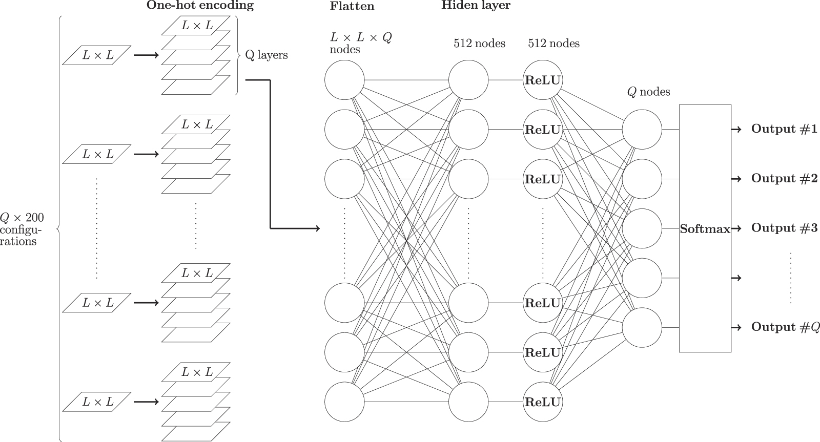
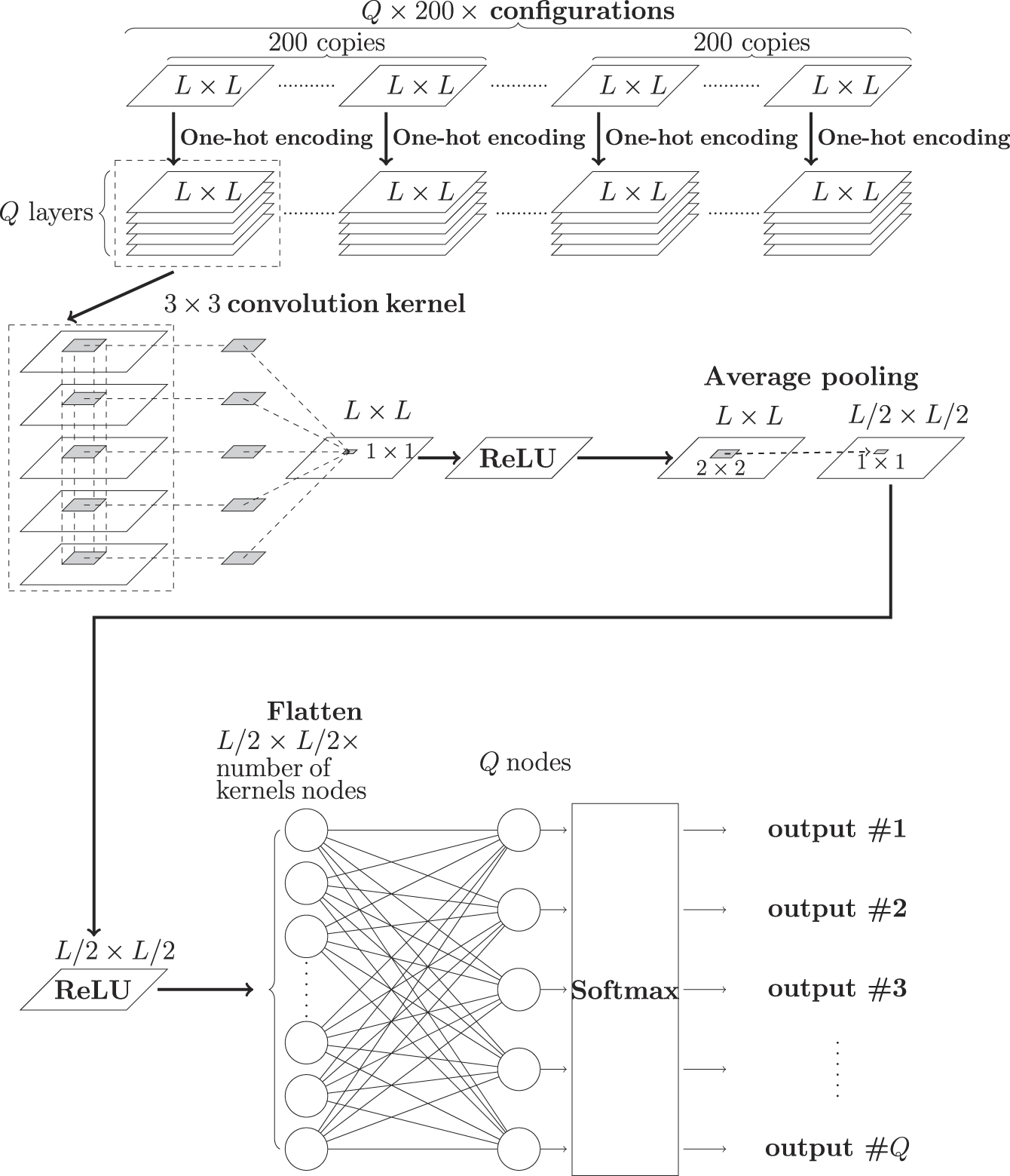
Since we would like to understand whether the simplest deep learning NN (multilayer perceptron, MLP) is capable of detecting the critical point, the supervised NN considered in our investigation consists of only one input layer, one hidden layer of 512 independent nodes, and one output layer using the publicly available NN libraries keras and tensorflow [51, 52]. The algorithm, optimizer, and loss function we employ for the calculations are minibatch, adam, and categorical cross entropy, respectively. L₂ regularization is applied as well to avoid overfitting. The activation functions considered are ReLU and softmax. The details of the constructed MLP, including the steps of one-hot encoding and flatten (and how these two processes work) are shown in figure 1. For comparison, calculations using the convolutional neural networks built in [27], which is depicted in figure 2, is conducted here as well. In addition, for the 3D model, computations using various batch size, nodes, copies of the pre-training set (defined later), and epoch are conducted as well. Moreover, the weights obtained in the training processes which minimize the loss function are recorded and are used in later calculations. Finally, to understand the impact on the output results from the initial values of weights as well as other steps performed in the training stage, several sets of random seeds are used in the investigation. For the studied 2D antiferromagnetic model, all the outcomes obtained with various random seeds will be considered in determining the final results associated with this model.

Zoom In Zoom Out Reset image size

Zoom In Zoom Out Reset image size

3.2. Training set and output labels for the 3D model

Regarding the training set used for the 3D five-state ferromagnetic Potts model on the cubic lattice, we will follow the idea considered in reference [27], namely the employed training set consists of 200 (or any suitable number) copies of the corresponding theoretical ground state configurations. The expected ground state configurations for 3D five-state ferromagnetic Potts model on an L × L × L cubic lattice are obtained by letting the Potts variables on all the lattice sites take the same (positive) integer from {1, 2, 3, 4, 5} as their values. Consequently, there are five ground state configurations. The associated labels for these five ground state configurations are the basis vectors of five-dimensional (5D) Euclidean space. While not being unique, clearly one can construct an one to one correspondence between the five ground state configurations and the basis vectors of 5D Euclidean space. One of such correspondence is shown in figure 3. These five ground state configurations will be named pre-training set in this study. Finally, we would like to emphasize the fact that when constructing the pre-training set, all the allowed Potts variables should be used.

Zoom In Zoom Out Reset image size

3.3. The expected output vectors for the 3D model at various T

With such a set up of pre-training set, it is expected that at extremely low temperatures, the norm (R) of the NN output vectors are around 1 since most of the Potts variables take the same positive integer Q₁ as their values. As a result, one component of the associated output vector has much larger magnitude than that of the others. The norm of such a vector clearly is around 1.

As the temperature arises, some Potts variables begin to obtain other positive integers than Q₁. Consequently, the magnitude of norm of the output vectors diminishes with T. When T ⩾ T_c, the norm of NN output vectors are around its minimum value $1/\sqrt{5}$. This is because there is an equal probability that each integer in {1, 2, 3, 4, 5} is the value of any Potts variables. The cartoon plots shown in figure 4 demonstrates how the Potts configurations and the corresponding output vectors change with T. Based on this scenario of R versus T, T_c can be estimated to lie within the temperature window at which R decreases rapidly from 1 to $1/\sqrt{5}$. Indeed such a method is shown to be able to determine T_c with high precision in reference [27]. For a more detailed introduction to this approach of using the theoretical ground state configurations as the training set, including its validation, we refer the readers to reference [27].

Zoom In Zoom Out Reset image size

3.4. Training set and output labels for the 2D model

Similar to the strategy introduced in the previous subsection, here we will employ the expected ground state configurations as the pre-training set for the NN study associated with the considered 2D system. Unlike the ferromagnetic Potts model, any two nearest neighboring Potts variables for the ground state configurations of 2D Q-state antiferromagnetic Potts model differ from each other. As a result, there are tremendous number of such configurations when Q ⩾ 3. We construct 6, 18, and 36 expected ground state configurations of the 2D three-state antiferromagnetic Potts model and use these configurations as the pre-training sets. The unit blocks (2 by 2 lattices and their Potts variables) for the built 6 configurations are shown in figure 5, and configurations on larger lattices are obtained by multiplying any of these 6 unit blocks by itself several times in both the x- and y-direction (the associated labels which will be introduced shortly are demonstrated in figure 3 as well). Using these pre-training sets, the actual training sets are a multiple copy (here we use a factor of 200) of the pre-training sets.

Zoom In Zoom Out Reset image size

The output labels used here for the pre-training sets follows exactly the ones in the previous subsection related to the 3D five-state ferromagnetic Potts model. For instance, for the pre-training set consisting of 6 configurations, the corresponding labels are the basis vectors of six-dimensional Euclidean space. Clearly, similar to the case of ferromagnetic Potts model, one can map these 6 configurations in the pre-training set onto the 6 basis vectors of six-dimensional Euclidean space in an one to one manner (this map is not unique as well). The same construction rule applies when 18 or 36 configurations are considered as the pre-training set, see figure 6 for part of the pre-training sets consisting of 18 and 36 configurations.

Zoom In Zoom Out Reset image size

Remarkably, although in this study only very little information of the whole ground state configurations are employed as the training sets, as we will demonstrate shortly, the built NN with the designed training sets and labels is capable of showing convincing evidence that the phase transition of the investigated 2D three-state antiferromagnetic Potts model occurs only at zero temperature as the theory predicts.

To generate configurations of the studied 2D and 3D Potts models, which will be used in the testing stages of the NN procedures, Swendsen and Wang algorithm [43], Wolff algorithm [48], as well as Swendsen–Wang–Kotecky algorithm [44, 45] are adopted. Particularly, Potts configurations are stored once in every thousand (or two thousand) Monte Carlo sweeps after the thermalization, and ten thousand (or two hundred thousand) 3D ferromagnetic Potts configurations as well as one thousand 2D antiferromagnetic Potts configurations are produced. These configurations are used in obtaining the results presented here.

4.1. Results of 3D five-state ferromagnetic Potts model

4.1.1. The Monte Carlo results

In figure 7, the energy density E as a function of MC sweep (top panel), and the histogram of the magnetization density ⟨|m|⟩ (bottom panel) at a temperature close to T_c for the 3D five-state ferromagnetic Potts model on the cubic lattice are shown. The outcomes are obtained with L = 16 and β = 0.689. The phenomenon of tunneling between two values clearly appear in the top panel of the figure. In addition, two peaks structure shows up as well in the bottom panel of figure 7. These are the features of a first order phase transition. In other words, our Monte Carlo data confirm the theoretical prediction that the phase transition of 3D five-state ferromagnetic Potts model on the cubic lattice is discontinuous.

Zoom In Zoom Out Reset image size

4.1.2. The NN results

The norm R of the output vectors as functions of T for the 3D five-state Potts model on the cubic lattice are demonstrated in figure 8. The vertical dashed line which appears in the figure is the expected T_c. These results are obtained on 12 by 12 by 12 lattices. Moreover, for a fixed T four calculations using different parameters of random seeds, batch size, copies of the pre-training set, and epoch are conducted and all the obtained resulting R are shown in the top panel of figure 8. The outcomes in figure 8 indicate that R is very stable with respect to the tunable variables associated with NN. In addition, as can be seen from the figure as well as that of figure 9 which includes the outcomes of L = 16, the magnitude of R decreases rapidly in the temperature region close to the theoretical T_c. Based on this result and that of reference [27], it is beyond doubt that for Q-state ferromagnetic Potts model, the associated T_c can be precisely estimated to lie within the temperature window at which the magnitude of R drops sharply from 1 to 1/$\sqrt{Q}$.

Zoom In Zoom Out Reset image size

Zoom In Zoom Out Reset image size

Figure 10 shows the history of R for the 3D five-state ferromagnetic Potts model on the cubic lattice at a temperature T near T_c. The outcome is obtained with L = 16 and β = 0.689. A clear tunneling obviously appears in the figure. As a result, the studied phase transition is first order. In other words, the NN constructed here, which consists of only one input layer, one hidden layer, and one output layer, is capable of not only locating T_c precisely, but also determining the nature of the phase transition of the investigated model. It is anticipated that the built NN can carry out similar calculations with success for general Q-state ferromagnetic Potts models in any dimension and on any lattice geometry.

Zoom In Zoom Out Reset image size

Apart from the results determined by MLP, we have additionally carried out calculations using the constructed CNN demonstrated in figure 2. Both the outcomes of R associated with MLP and CNN for L = 8 and L = 12 as functions of T are shown in figure 11. In the figure the vertical dashed and horizontal solid lines represent T_c and $1/\sqrt{5}$ respectively. Here again $1/\sqrt{5}$ is the expected value for R when the system size goes to infinity. Based on the outcomes shown in figure 11, both MLP and CNN successfully (and accurately) determine the location of T_c.

Zoom In Zoom Out Reset image size

We have also calculated the R for temperatures close to the theoretical T_c. The L = 16 results resulting from both the MLP and the CNN are depicted in figure 12. Close to the vertical line, which is the established T_c, the variations of R are large. Since efficient cluster type algorithm is used for the simulations, such a result can be interpreted as a signal for a first order transition (this can be derived from the feature of tunneling between two channels for a first order phase transition). It is also intriguing that the temperature region where the variations of R become large is slightly above the established T_c in the literature (vertical line in figure 12). This small discrepancy can be attributed to different approaches as well as algorithms employed in calculating T_c.

Zoom In Zoom Out Reset image size

Finally, the history of R at β = 0.689 obtained from CNN is shown in figure 13. Similar to situation of MLP, R tunnels between two values with Monte Carlo sweeps, which again is a clear message that the phase transition is first order.

Zoom In Zoom Out Reset image size

4.2. Results of 2D three-state antiferromagnetic Potts model

4.2.1. The Monte Carlo results

In figure 14 the staggered magnetization density m_s as functions of temperature T for the considered 2D three-state ferromagnetic Potts model on the square lattice are presented. In particular, outcomes corresponding to various L are shown in the figure. The results in the figure demonstrate that for every finite L, the magnitude of its corresponding magnetization diminishes as T rises and eventually at high temperature m_s reaches a saturated value which is anticipated to go to zero when L → ∞. Moreover, for the simulated box sizes, the curves shown in the figure do not intersect among themselves. Such a scenario is interpreted as the phase transition takes place at zero temperature, namely the system is always in the disordered phase at any T > 0.

Zoom In Zoom Out Reset image size

4.2.2. The NN results

The NN outcomes of R as functions of T for various training sets (using 6, 18, and 36 constructed configurations as the pre-training sets) are shown in figures 15–17, and the shown data are obtained using ten results. In particular, each of these results is calculated with its own set of random seeds which is different from that of the others. These figures, which are obtained using different training sets, all demonstrate similar characteristics as that of m_s (figure 14). Specifically, the T–R curves of various L have the trend that the magnitude of R decrease monotonically with T. In addition, for every employed training set, the associate T–R curves do not intersect among themselves except those of larger L, which can be interpreted as the size convergence of the NN outcomes. The horizontal solid line located at the bottom of figure 15 is the expected value of R (which is $1/\sqrt{6}$) at any finite temperature when L → ∞. It is anticipated that as L increases, the associated R will approach $1/\sqrt{6}$ even at the low temperature region.

Zoom In Zoom Out Reset image size

Zoom In Zoom Out Reset image size

Zoom In Zoom Out Reset image size

We would like to point out that for the results of using 18 configurations as the pre-training set (i.e. figure 16), in the high temperature region R of L = 64 are slightly above that of L = 32 (not within statistical errors). We attribute this to the systematic uncertainty due to the tunable parameters of NN that are not taken into account here. Nevertheless, considering the similarity between the results of NN and MC (i.e. figures 14–17), the outcomes of NN provide convincing numerical evidence that the phase transition of 2D three-state antiferromagnetic Potts model on the square lattice occurs at zero temperature.

When compared with that of the studied 3D model, the NN outcomes of the 2D three-state antiferromagnetic Potts model have (much) larger uncertainties. Indeed, for the calculations using various random seeds, while the variation among the resulting R associated with the considered 3D model is negligible, the uncertainty of R related to the studied 2D model has sizable magnitude. Similarly, other tunable parameters in the used NN such as the batch size have certain impact on the outcomes of R of the antiferromagnetic system. We further find that in order to obtain results consistent with that determined from Monte Carlo simulations, the ratio p between how many objects in the training set and the considered batch size has to be a number with moderate magnitude. Since p is associated with the independent parameters during the optimization procedure, too many or too few free parameters will lead to not satisfactory outcomes from the optimization considering the limitation of the algorithm employed in this process.

Using 18 configurations as the pre-training set, the NN outcomes of R for various T and L obtained using batch sizes 40, 80, 160, and 320 are shown in figure 18 (from top to bottom). As can be seen in that figure, when batch size is 40 the corresponding data of L = 128 lie well above those of L = 32, 64 in the high temperature region. This is in contradiction with the Monte Carlo results. As the batch size increases, the trend of R versus T for various box sizes L become more and more similar to that of MC. Finally, the outcomes shown in the bottom panel of figure 18 which is calculated with batch size 320 are consistent, at least qualitatively, with that of MC. Our investigation of 2D three-state antiferromagnetic Potts model on the square lattice indicate that cautions have to be taken, when NN techniques are considered to study physics systems having highly degenerated ground state configurations.

Finally, we would like to emphasize the fact that the results shown in each of figures 15–17 are obtained using the same variables of NN for all the considered box sizes L = 8, 16, 32, 64(128). It is likely that the most suitable parameters associated with NN for various L could be different. In other words, for complicated systems, carrying out certain fine tuning to search appropriate parameters of NN may be required in order to reach the right signals of physics.

Zoom In Zoom Out Reset image size

In this study we investigate the phase transitions of 3D five-state ferromagnetic Potts model and 2D three-state antiferromagnetic Potts model, using both the Monte Carlo calculations and techniques of NN. The NN considered here are MLP and CNN. The employed MLP has the simplest deep learning structure, namely it consists of one input layer, one hidden layer, and one output layer. In addition, the used CNN is constructed following the one outlined in [27]. Finally, unlike the conventional approach of using data generated by numerical methods for the training, in our study we employ full or part of the theoretical ground state configurations as the (pre-)training sets.

The conventional training of an NN typically requires the use of actual data points. In particular, the knowledge of the critical point (T_c) is essential to study the associated phase transition using the standard approach of NN methods. Our strategy for the training process has the advantage that information of T_c is not necessary to carry out the investigation and very little computation effort is needed for generating the training sets. The magnitude of the output vectors R is shown to be the relevant quantity to locate the critical points as well as to determine the nature of the phase transitions.

Remarkably, the NN results related to the studied 3D models obtained here imply that even a simplest NN of deep learning can lead to highly accurate determination of T_c. Furthermore, the quantity R used here is as efficient as that typically considered in the traditional methods when it comes to decide the nature of the considered phase transitions. Interestingly, the tunneling phenomena in figures 7 and 10 indicate that, whenever E reaches the results of large numerical values, R obtains the outcomes with small magnitude and vice versa. In other words, R and E are complementary to each other and R indeed reflects the correct physics.

For the 2D three-state antiferromagnetic Potts model, we have carried out the NN investigation using 6, 18, and 36 theoretical ground state configurations of this model as the (pre-)training sets. While the resulting NN outcomes with certain constraints on the tunable parameters are consistent with the Monte Carlo results, it is subtle to reach the correct physics from the NN calculations. Indeed, as we have demonstrated here, the variation among NN results obtained with different random seeds and batch size are not negligible. In particular, the ratio of the number of training objects and the batch size plays a crucial role in obtaining outcomes having the right signals of physics. In summary, one has to pay special attention when models having highly degenerated ground state configurations are investigated using the NN method. For such cases, certain fine tuning to search appropriate parameters of NN may be required in order to observe the correct physics.

We would like to emphasize the fact that since the results presented here imply that only partial information is needed to obtain the correct physics, at least qualitatively, it is likely that with moderate modifications, the strategy considered here is applicable to classical systems with continuous variables and quantum spin models. For spin-1/2 antiferromagnetic Heisenberg model, the corresponding classical ground states consists of two configurations. Using these two classical ground state configurations as the training set, our preliminary results of investigating the quantum phase transition associated with the three-dimensional plaquette model considered in reference [53] are shown in figure 19. While the NN data are represented by the down-triangle symbols in the figure, the solid circles stand for the outcomes of $1/\sqrt{2}+1-\text{NN}\;\text{data}$. The consideration of the new data set (of solid circles) is motivated by approximating the trend of R as a function of g in the critical regime linearly. With such an idea, the g_c should be the g associated with the middle point of the mentioned linear approximation. As a result, the g_c can also be determined by the intersection of the curves represented by the down-triangle and solid circle symbols. With such a criterion, the estimated g_c is around 4.0 which is in reasonable agreement with the one calculating using the data of reference [53]. Since the two classical ground state configurations used for the training are not even the true ground states of the considered quantum spin system, it is plausible that the applicability of the method employed in this study is beyond what one would intuitively expected.

Zoom In Zoom Out Reset image size

By applying this described strategy to the L = 12 data of the 3D five-state Potts model, we arrive at figure 20 which unambiguously confirms the claim(s) made in the previous paragraph. We would like to point out that since the phase transition for the 3D five-state Potts model is first order, the effectiveness of determining T_c by the intersection of two data sets associated with R requires further investigation. Nevertheless, the results shown in figures 19 and 20 indicate that this method is promising.

Zoom In Zoom Out Reset image size

To conclude, here we reconfirm the validity of the training approach considered in reference [27]. In particular, we succeed in applying this method to the study of the phase transition of 2D three-state antiferromagnetic Potts model on the square lattice. This phase transition takes place at zero temperature and may be difficult to detect using the conventional NN training procedure. It will be interesting to examine whether the method employed in this study is capable of precisely calculating other relevant physical quantities at phase transitions, such as the critical exponents.

While the NN calculations conducted in this study is for a well-known statistical model, the usage of the ideas employed here is beyond what have been obtained. As already being pointed out in the introduction, the application of AI methods in the majority fields of science requires the use of real data points as the training sets. The outcomes obtained in this study indicate that solely AI techniques, without any input of real data, can successfully reach correct physical results. This encourages applying the approaches along the spirit of this study to more complicated systems, which can be accomplished by the following procedures. Assuming a theory is proposed to be the relevant theory describing a real material, one can examine whether this is the case or not by first carrying the training with only the theoretical inputs (no experimental data required), followed by using the real data for the testing stage. Finally, by inspecting the output results, one can determine if the proposed theory is appropriate for the targeted material or not.

The first three authors contributed equally to this project. Partial support from Ministry of Science and Technology of Taiwan is acknowledged.