


Abstract
Implementing a positive correlation between the natural frequencies of nodes and their connectivity on a single star graph leads to a pronounced explosive transition to synchronization, additionally presenting hysteresis behavior. From the viewpoint of network connectivity, a star has been considered as a building motif to generate a big graph by graph operations. On the other hand, we propose to construct complex synchronization dynamics by applying the Cartesian product of two Kuramoto models on two star networks. On the product model, the lower dimensional equations describing the ensemble dynamics in terms of collective order parameters are fully solved by the Watanabe–Strogatz method. Different graph parameter choices lead to three different interacting scenarios of the hysteresis areas of two individual factor graphs, which further change the basins of attraction of multiple fixed points. Furthermore, we obtain coupling regimes where cluster synchronization states are often present on the product graph and the number of clusters is fully controlled. More specifically, oscillators on one star graph are synchronized while those on the other star are not synchronized, which induces clustered state on the product model. The numerical results agree perfectly with the theoretic predictions.
Export citation and abstract BibTeX RIS

Original content from this work may be used under the terms of the Creative Commons Attribution 3.0 licence. Any further distribution of this work must maintain attribution to the author(s) and the title of the work, journal citation and DOI.
1. Introduction
A broad range of example systems shows synchronization properties as the interaction between units change, e.g. birds flocking, male fireflies flashing together, heart beating of mother and fetal, neurons in the brain, cardiac and respiratory system [1, 2]. One of traditional models to simulate synchronization dynamics is the Kuramoto phase oscillator model, which still attracts much attention in the literature [3–6].
In the traditional Kuramoto model, as the coupling strength increases, a transition from an incoherent to a coherent state takes place generically at a critical value of λc, after which the interacting units follow the same dynamical behavior. This macroscopic appearance of synchronization is often described by an order parameter r which is normalized to r ∈ [0, 1]. Namely, a small value of r ≈ 0 corresponds to an incoherent state, while a large value of r close to 1 indicates a high degree of synchrony. Both the natural frequencies of oscillators and the coupling strength determine the synchronization transition properties. As first pointed in [7], in most cases the transition is second-order like, with the order parameter r growing continuously when the coupling strength passes the critical threshold λc of synchronization [8]. On the other hand, abrupt discontinuous transitions to synchronization have been recently reported in both all-to-all coupling [3, 9] and complex network topologies [10–15] where an infinitesimal variation of the coupling strength gives rise to a macroscopic explosive transition to synchronization. In the study of explosive sync, the transition from an initially incoherent to a coherent state is referred to as forward continuation curve when the coupling strength is progressively increased and the corresponding critical coupling is termed as  . In contrast, the desynchronization transition from an initially coherent to an incoherent state is called backward continuation curve when the coupling is decreased and the critical coupling is denoted as
  . In addition, a clear hysteresis area has been observed between these synchronization and desynchronization processes, which is further denoted as
  .
.
Recently, star graphs have been applied to understand the global explosive behavior of the order parameter r which shed insights for other cases of more general heterogeneous network settings [10, 13, 16]. The two fundamental results of explosive synchronization (discontinuity and hysteresis) have been delineated by the Watanabe–Strogatz (WS) approach [17, 18]. More specifically, the exact nonlinear equation for the order parameter r of the high dimensional coupled system has been explicitly obtained and the different synchronized states correspond to different steady states of the equation. Furthermore, different stability conditions of coexisting fixed points in the parameter space lead to the hysteresis behavior and the discontinuous transitions in both the forward and backward continuation curves [16].
From the viewpoint of network topologies, star graphs are considered as building motifs to generate a big graph by several graph operations, e.g. Cartesian product, direct tensor product and strong product [19, 20]. For example, the Cartesian product of graphs is a commutative, associative binary operation on graphs [21]. It has many useful properties, most of which can be derived from the factors. Furthermore, several multilayer network properties have been obtained by graph product operations [20]. On the other hand, from the viewpoint of dynamics on top of networks, it remains largely undisclosed that the synchronization process is obtained by similar graph product operations except some discussions on eigenspectra [22, 23]. In our work [24], we have provided a novel framework to obtain a canonical Kuramoto model by the Cartesian product operation from two independent factor graphs. In this earlier work, we focused on the Cartesian product for two basic network graphs of star and ring where we found a mixture state of both an explosive transition to sync in the forward curve and a continuous desynchronization transition in the backward curve. This mixture state of synchronization transitions cannot be easily observed in a single factor graph. However, the lower dimensional equations for the order parameters of the Cartesian product model have not been discussed in the literature.
In this work, we provide a more general dimension reduction treatment of the WS ansatz to the Cartesian product model, obtaining fully solved lower dimensional dynamical solutions of multiple fixed points for the order parameters. The stability of each fixed point has been obtained by a linear analysis. Comparing to the case of a single star graph, the results are richer depending on the interaction between the hysteresis areas of the two independent factor stars. In addition, cluster synchronization solutions have been obtained for the product model. A cluster synchronized state represents that the network evolves into subsets of oscillators in which members of the same cluster are synchronized, but members of different clusters are not [25, 26]. Together with Chimera states [27–29], cluster synchronization is one of most interesting partial synchronization scenarios that has attracted both theoretical and experimental studies [30, 31]. Recently, a computational group theory has been developed to characterize the emergence and stability conditions of cluster synchronization [26]. More specifically, one has to identify the set of symmetries of the network of interest by discrete algebra routines [25] or by approximation techniques when there are system parameter mismatches [32, 33]. Then the nodes of the network are partitioned into M clusters, which yields disjoint sets of nodes when all of the symmetry operations are applied to permute one from the other. Importantly, the dynamics of oscillators in each disjoint set is essentially unchanged by the permutations, forming a cluster of synchronized oscillators. Once the clusters are identified, the stability of the clusters can be further analyzed by the corresponding variational equations of the system. Differently from the literature, we emphasize that the proposed cluster synchronized behavior in this work are synthetic states that are constructed from the dynamics of two independent subgraphs by means of Cartesian graph operation, which therefore provides a novel 'bottom-up' framework to generate more complicate dynamics encountered in complex systems.
The outline of this paper is as follows: in section 2, we introduce the Cartesian product model from two independent star graphs and provide the WS ansatz. In section 3, we show the steady state solutions of the ensemble order parameters and their respective stability conditions. Numerical simulation are presented in section 4. Finally, our main conclusions are summarized in section 5.
2. Cartesian product of two Kuramoto models on stars
We consider the dynamics of two independent star networks of N1,2 leaf nodes and a central hub. The degree of a node is the number of connections it receives. So, the degree of the leaf nodes equals one and the degree of the central hub equals N. The equations of motion are described by

and

where ω1,2 is the natural frequency of the leaves, λ is the overall coupling strength, and β1,2 is a parameter controlling the frequency mismatch between the hub and the leaves [16]. In this model, β1,2 > 1 mimics a positive correlation between the hub's natural frequency and its degree, i.e. the hub of larger degree has a larger frequency than that of a leaf node [10, 13]. The parameter β1,2 helps to understand a more general effect besides the network degrees. In addition, we consider a lower dimensional dynamics in the thermodynamic limit  , so the normalization is necessary to make sense of the limit, otherwise the hub would rotate infinitely fast.
Following [16], we introduce the phase differences as

In addition, the order parameters of the two independent networks are defined as

where is the bold font i is for the imaginary unit throughout this paper. Then the original models (equations (1), (2)) are rewritten as the following compact forms


For individual factor graphs, the order parameters of equations (4) represent the mean-field coupling terms in the above compact equations (5), (6).
The Cartesian product of the two stars G1 and G2 are schematically shown in figure 1. Meanwhile, we use the notation  to represent the index of node on the product
  . In addition, on the Cartesian product graph, the phase of the node
  is defined as
  . Note that the definition of the phase of the node on the product graph as the summation of the respective phases on the factor subgraphs yields the canonical equations of the Kuramoto model on
  [24]. Furthermore, with the commutative and associative properties of the phase summation of the Cartesian product operation, we easily generalize the present results to the case of n factor subgraphs [24].
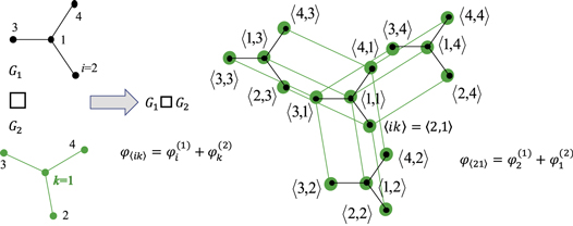
Figure 1. Schematic illustration of Cartesian product of two stars. Phase of node  on
on  is defined as
  . An example is shown by node index i = 2 of G1 and k = 1 of G2, which is denoted by
  on
on  .
.
Download figure:
Standard image High-resolution imageIn addition, the order parameter of the Cartesian product model is defined as

In a full analogy, we note that the above definition of Z(t) preserves the mean-field coupling properties. In the present framework of phase summation, the right-hand side of equation (7) can be further expanded, which yields Z(t) = z1(t) z2(t). Namely, the order parameter on  is the product of two factor graphs. The summation rule of phases can be generalized to the case of more than two factor graphs straightforwardly, while preserving that the order parameter Z is the product of subgraphs. For instance, given three factors G1, G2 and G3, the order parameter R of the product
  is R = R1R2R3 [24].
With the above phase definition, the time derivatives of the phases  on the Cartesian product
  are
are


where f* are the complex conjugates of f. The f and g1,2 are further defined as

Note that, in equation (9), the term (1 − β1)ω1 + (1 − β2)ω2 represents the natural frequency of the oscillator on the product  , while the rest terms are the coupling [24].
The above phase equation (11) has exactly the form such that the WS ansatz can be applied. The WS approach [34, 35] is applicable for systems of identical oscillators driven by a common force. More specifically, in the product model of equation (11), identical oscillators g1 + g2 are driven by the arbitrary complex  , where c.c. are the complex conjugates.
Next, the basic idea is to expand the model system (equation (11)) in terms of the global variables of z1, z2 and Z. Therefore, we first consider the relationship


Furthermore, in the formulation presented in [17, 18], we need to introduce a series of Möbius transformations that expand the exponential functions in the above polynomial in terms of the order parameters. Importantly, we introduce

Similar Möbius transformations of other terms have been included in the appendix. Note that the variables of ξi,k are constants. Remarkably, in the case of a uniform distribution of ξi,k, the global variables α1,2 and ξi,k do not enter the equation for z1,2 and Z [16, 17]. Thus, the equation for Z is a closed equation that fully describes the dynamics of the system (equation (11)), and therefore in the following, we focus on the discussion on Z only. Furthermore, it has been shown in [36, 37], for  and the uniform distribution of constants of motion ξi,k, the WS variables z1, z2 coincide with the local Kuramoto mean-field, namely yielding the Ott–Antonsen (OA) ansatz [38–40].
Putting these Möbius transformations into the two sides of equation (14), we obtain the following relationship by equalizing the non-exponential terms of the two sides of the equations (13), (14).

As it has been proved in [24], the order parameter Z of the Cartesian model is the product of the order parameters of the two independent factors, namely, Z = z1z2. Then, we have  . Therefore, in terms of the global variables Z, the phase equation equation (11) is expressed as

Considering the definition of the order parameter  (equation (7)), we obtain the following two nonlinear coupled equations for the global order parameter in the complex plane


3. Steady states of the product model
There are three steady states of the nonlinear coupled system (equations (18), (19)), namely,
- 1.Full synchronization of r1 = r2 = 1,
- 2.Non-synchronization of
 and ,
and , - 3.Cluster synchronized state of r1 = 1 and .


In the following subsections, we get the explicit expressions for the global order parameter Z of the Cartesian product model in terms of Z = z1z2. To this end, we first denote the forward critical coupling threshold values for the two independent factors following the notations of [16]:

and two backward critical coupling thresholds

In addition, we consider β1,2 > 1 which implement positive correlations between the node frequency and its associated number of connections [16]. In other words, the following inequalities do hold always

which further ensure that the hysteretic areas exist for both independent star graphs, namely,  and
and  .
.
3.1. Full synchrony for the product model r1 = r2 = 1
In this case, equations (18), (19) are simplified as


Since β1,2, ω1,2 and λ are positive, the solutions Φ1,2 exist only if  and
and  . Note that this corresponds to the existence of the phase locking manifold [13], which therefore yields the critical coupling for the backward continuation curves as
  and
and  , respectively. In this case, the solutions of z1 and z2 are easily obtained as


Furthermore, keeping in mind the condition of  , and therefore the solution of the product model has the following expression

3.2. Non-synchrony for the product model and


Inserting the steady states of  and
and  into equations (18), (19), we obtain


Considering the fact that  or
or  , we get


Note that both z1,2 exist only if  hold. Furthermore, both '+' and '−' are possible if (β1,2 − 1)ω1,2 ≤ (β1,2 + 1)λ, while '−' is possible if (β1,2 − 1)ω1,2 > (β1,2 + 1)λ. In consequence, the expression of the global order parameter of the product model Z = z1z2 has several different cases while considering
  . Depending on the relationship between
  or
or  , we will have different solutions for Z and the details are omitted here for the simplification purpose, which will be summarized in section 3.4.
3.3. Cluster synchronized states of r1 = 1 and

We focus on the discussion on the case of r1 = 1 and  , while the symmetric case of r2 = 1 and
  shows a full analogy. In this case, we have the following two equations in order to obtain the steady states, namely


From equation (32), we get

From equation (33), we obtain

Both '+' and '−' are possible for z2 if (β2 − 1)ω2 ≤ (β2 + 1)λ, while only '−' is possible for z2 if (β2 − 1)ω2 > (β2 + 1)λ. The order parameter Z for the product model is Z = z1z2 again with different expressions depending on β1,2 and ω1,2, which will be summarized in section 3.4.
3.4. Intermediate summary of steady states
Note that the critical coupling thresholds  and
and  subdivide the coupling strength into five subintervals. All solutions for Z of the product model have been summarized in the following when
  . When switching the notations of the two factor subgraphs G1 and G2, we obtain the case of
  which is in a full analogy as we summarized below. Therefore, we only focus on
  . In this case, we further have three subcategories as illustrated in figure 2, depending on the critical value of
  . From the viewpoint of hysteresis areas of
  and
and  , these three subcategories correspond respectively to
  ,
,  , and
, and  .
.

Figure 2. Schematic illustration of different Z solutions, depending on the three choices of  . Namely, (a)
  , (b)
, (b)  , and (c)
  . The critical coupling threshold values of the product model in each case have been highlighted by squared notations.
Download figure:
Standard image High-resolution imageAll possible solutions are expressed in terms of the product of the two subgraphs, namely, Z = z1z2. The respective existence regimes of Z are illustrated in figures 2(a)–(c).


Note that in the case of figure 2(a), the solutions of  ,
,  ,
,  ,
,  ,
,  and
and  do not exist. Additionally, the solutions
  correspond to four synchronous states, showing different stability conditions as we summarize in the next section.
3.5. Linear stability analysis
Accordingly, we obtain the stability of each fixed point (equations (36)–(43)). Therefore, we first obtain the Jacobian matrix of the system (equations (18), (19)) which is expressed as

where f and g are the right-hand side of the system (equations (18), (19)). The elements of J are the following:


The stability is studied by inserting each steady state solution into the trace and determinant of the Jacobian matrix (equation (45)). Due to the lengthy of the derivation, we only summarize the stability of the fixed points and the corresponding physical meaning according to the three subcategories as illustrated in figures 2(a)–(c), which are respectively shown in tables 1–3.
Note that the fixed points of  correspond to four synchronous states of different stabilities which are determined by the products from
  and
and  . Taking figure 2(a) as an example (table 1),
  is a stable sink if both
  and
and  are positive real values, and
  is an unstable source if both
  and
and  are negative real values. On the other hand,
  is either a stable sink or an unstable source if
  is a positive real value and
  is a negative real value. Respectively,
  is either a stable sink or an unstable source if
  is a negative real value and
  is a positive real value. The annotations of other two cases of tables 2 and 3 have similar stability conditions.
Table 1. Fixed points of the order parameters with their stability and meaning for figure 2(a).
| Fixed point | Stability | Existence region | Physical meaning |
|---|---|---|---|

|
Sink |

|
Coherent state |

|
Source |

|
Coherent state |

|
Sink or source |

|
Coherent state |

|
Sink or source |

|
Coherent state |

|
Center |

|
Asynchronous state |

|
Saddle |

|
Separatrix |

|
Center |

|
Cluster sync |

|
Saddle |

|
Separatrix |
Table 2. Fixed points of the order parameters with their stability and meaning for figure 2(b).
| Fixed point | Stability | Existence region | Physical meaning |
|---|---|---|---|

|
Sink |

|
Coherent state |

|
Source |

|
Coherent state |

|
Sink |

|
Coherent state |

|
Source |

|
Coherent state |

|
Center |

|
Asynchronous state |

|
Saddle |

|
Separatrix |

|
Saddle |

|
Separatrix |

|
Saddle |

|
Separatrix |

|
Center |

|
Cluster sync |

|
Saddle |

|
Separatrix |

|
Saddle |

|
Separatrix |

|
Center |

|
Cluster sync |
Table 3. Fixed points of the order parameters with their stability and meaning for figure 2(c).
| Fixed point | Stability | Existence region | Physical meaning |
|---|---|---|---|

|
Sink |

|
Coherent state |

|
Source |

|
Coherent state |

|
Sink |

|
Coherent state |

|
Source |

|
Coherent state |

|
Center |

|
Asynchronous state |

|
Saddle |

|
Separatrix |

|
Saddle |

|
Separatrix |

|
Saddle |

|
Separatrix |

|
Center |

|
Cluster sync |

|
Saddle |

|
Separatrix |

|
Saddle |

|
Separatrix |

|
Center |

|
Cluster sync |
4. Numerical results
Now, we follow mainly the simulation routines as presented in [16, 24] and have numerically simulated the model equations (1), (2) by using a fourth order Runge–Kutta integrator with the integration step h = 0.01. When the coupling λ = 0, the initial conditions (ICs) are uniformly distributed over the interval [−π, π]. Then the coupling is increased by a step size Δλ = 0.02 and the ICs for the coupling λ + Δλ are the final states when coupling equals to λ as suggested in [10, 13]. The first T = 105 steps are discarded as transients and the next T iterations are used to estimate the order parameter. We consider the time average of the order parameter  . Note that this average is useful as the asynchronous fixed points of the order parameter are centers, and so the order parameter in the asynchronous regime shows oscillatory behavior.
There are two equivalent ways to implement the dynamics of the Cartesian product model: (i) We simulate G1 and G2 (equations (1), (2)) simultaneously, while phase dynamics of the product G1 G2 simply follows the Cartesian product summation rule of the corresponding phases. (ii) We simulate the Cartesian model equation (11), directly. The ODE integrator is performed for N1 + N2 phase oscillators in the former case, yielding a better computation efficiency than that of the latter case that is integrated for N1N2 oscillators. The additional requirement for the second simulation method is that we have to obtain the connectivity matrix of the product model, in particular, the adjacency matrix of
  is the Kronecker sum of the adjacency matrices of G1 and G2, namely,
  . Throughout this work, we have obtained the same results for these two slightly different ways of numerical simulations. In the examples below, we choose N1 = N2 = 100.
For a better understanding of the product effects on synchronization transitions, we choose the parameters such that both the forward and backward critical coupling thresholds of G1 do not vary among the three cases of figures 2(a)–(c), namely, β1 = 9, ω1 = 1.2, which yield  ,
,  , and
, and  . In the case of G2, we choose β2 and ω2 such that
  is fixed as 0.48, but
  is changed in such a way that, respectively, represents the three different regimes that are illustrated in figures 2(a)–(c). Note that our theoretical predictions obtained by the lower dimensional dynamics of the product model agree very well with the numerical simulations.
4.1. Case A of figure 2(a)
The first case of figure 2(a) is implemented by choosing parameters β2 = 3 and ω2 = 0.96, which yield  ,
,  , and
, and  , namely
  . In this case, the two hysteresis areas
  and
and  are well separated, leading to
  as shown in figures 3(a), (b). Therefore, on the product model
  , we observe two separated hysteresis areas as well, which are shown in figures 3(c), (d). In particular, starting from the incoherent state on G1 and G2 when λ = 0, the product model remains incoherent until
  . Note that when G2 experiences a jump at
  to the coherent state as zoomed in figure 3(d), however, the product model keeps incoherent since G1 is in an incoherent state. The forward continuation curve of the product model follows the incoherent solution of G1 until the critical coupling value of
  showing a jump to full synchronization. The backward continuation curve of the product model drops to an incoherent state at
  (figure 3(c)) because G1 loses synchronization first, while G2 keeps sync. Reducing the coupling λ further, G2 loses synchronization at
  , which yields the second drop to an even lower order parameter as zoomed in figure 3(d). From the viewpoint of global behavior, the hysteresis area of the product
  is determined by G1, namely,
  .
.
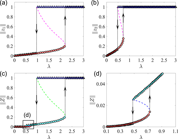
Figure 3. Theoretical and numerical results for the case figure 2(a), showing the order parameters for (a) subgraph G1, (b) subgraph G2, (c) product model  and (d) zooming of the rectangular area of (c). In the numerical simulations, the forward and backward continuation curves are, respectively, denoted by open circles and triangles. Theoretical solutions of stable steady states are represented by continuous lines while unstable solutions are denoted by dashed curves. The predictions for critical coupling threshold values are annotated by vertical arrows. The upward headed arrows are for the forward continuation while the downward headed arrows are for the backward curve. Line colors for steady states are:
  red bold;
  blue dashed;
  red dashed;
  pink dashed;
  light blue bold;
  green dashed;
  light blue dashed;
  black bold;
  blue bold.
Download figure:
Standard image High-resolution imageIn this case, the cluster synchronized states on the product model are found in both the forward and backward transition processes. In particular, in the coupling regime  of the forward transition, G1 is in an incoherent state, while G2 is in a coherent one, which yields the cluster sync states on the product model. In a full analogy in the coupling regime
  of the backward transition process, G1 is again incoherent while G2 is coherent, showing cluster sync dynamics. The microscopic details of these cluster synchronized states will be further illustrated in section 4.4.
4.2. Case B of figure 2(b)
The second case of figure 2(b) is implemented by choosing the parameters  and ω2 = 0.56, which yield
  ,
,  and
and  , namely
  . In this case,
  as shown in figures 4(a), (b), namely,
  is inside the hysteresis area of G1. In the forward transition process from an initially incoherent state at λ = 0, the product model
  remains an incoherent state until
  when G2 experiences the first jump at to a coherent state of
  (as shown in figures 4(c), (d)). Note, however, that when the coupling is further increased in the interval
  , the
, the  keeps the incoherent state since G1 is incoherent. The product model shows the second jump at
  when G1 is synchronized as well. The backward transition is the same as the case of figure 2(a), namely, the product model loses synchronization by the first jump down at
  , after which G1 is incoherent but G2 is coherent. Reducing the coupling further to
  , G2 loses synchronization leading to the second jump down to an even lower level of the incoherent state of the product model. The global hysteresis area of
  is determined by the subgraph G1,
 ![${S}_{{G}_{1}}=[{\lambda }_{c}^{{b}_{1}},{\lambda }_{c}^{{f}_{1}}]$](https://content.cld.iop.org/journals/1367-2630/21/12/123019/revision2/njpab5cc7ieqn201.gif) .
.

Figure 4. Similar caption as figure 3, but for the case figure 2(b). In the coupling regime  , the abnormal cluster synchronized states
  and
and  are respectively highlighted by filled diamond and triangle dots in (c), (d).
Download figure:
Standard image High-resolution imageIn the forward transition process on the product model, the cluster sync states are observed in the coupling regime  since G1 is incoherent while G2 is coherent. The cluster sync scenario for the backward transition process is the same as figure 2(a) in the coupling regime of
  , where G1 is incoherent but G2 is coherent.
The stability analysis of steady states of the product model suggests that there are further stable cluster synchronized solutions of  and
and  in the coupling regime
  , which are not easily observed by the previous traditional ways of implementing the forward transition process on both subgraphs G1 and G2 simultaneously (or the backward transition process respectively). In contrast, these clustered states are obtained by the product of the forward curve of G1 with the backward curve of G2 transition processes, which leads to the solution
  , or the product of the backward of G1 with the forward of G2 transition processes, which leads to
  . Both cluster sync solutions are, respectively, highlighted by filled diamond and triangle dots in figures 4(c), (d).
4.3. Case C of figure 2(c)
The third case of figure 2(c) is implemented by choosing the parameters  and
and  , which yield
  ,
,  and
and  , namely
  . In this case,
  as shown in figures 5(a), (b).

Figure 5. Similar caption as figure 3, but for the case figure 2(c). In the coupling regime  , the abnormal cluster synchronized solutions of
  and
and  are respectively highlighted by filled diamond and triangle dots in (c), (d).
Download figure:
Standard image High-resolution imageThis case shows a different forward transition process compared to the previous two cases. In particular, the product model  is incoherent until G1 experiences a jump at
  to a higher level of incoherent state that G1 is coherent but G2 remains incoherent. When the coupling is further increased to
  ,
,  is fully synchronized because G2 undergoes the second jump to synchronization. The backward transition process is the same as in the previous two cases of figures 2(a), (b) since both critical values
  and
and  are not affected. The product model loses sync by the first jump down at
  and then by the second jump at
  to a lower level of incoherent state. The global hysteresis area of
  is
is ![$[{\lambda }_{c}^{{b}_{1}},{\lambda }_{c}^{{f}_{2}}]$](https://content.cld.iop.org/journals/1367-2630/21/12/123019/revision2/njpab5cc7ieqn231.gif) . This size is larger than that of the single G1 subgraph because of the product effect from G2.
. This size is larger than that of the single G1 subgraph because of the product effect from G2.
In the forward transition process, the cluster synchronized states are observed in the coupling regime  since G1 is synchronized but G2 is not. Again because there are no changes for
  nor
nor  , the cluster sync scenario is observed in the coupling regime of
  of the backward transition process. Note again that the product model is obtained by performing the Cartesian operation on the forward continuation curves of G1 and G2 simultaneously (or the backward curves).
Furthermore, the stability analysis suggests further cluster synchronized solutions in the coupling regime of  which are similar to the results as presented in figure 4(d). In this particular coupling interval, we obtain the steady state of
  when performing the Cartesian product on the forward continuation process of G1 with the backward process of G2. On the other hand,
  is achieved by the product of the backward process of G1 with the forward process of G2, which are highlighted in figures 5(c), (d).
4.4. Microscopic views of cluster synchronized behavior
We have obtained cluster synchronized states in all three cases above. These states are generated in the coupling regime where one subgraph is synchronized, while the other subgraph is not. In this subsection, we numerically show the microscopic details of these states on the product model.
First, on the product model each node is denoted by  (equations (5), (6)). For an illustration purpose, we relabel the oscillators as
 ![$m=\{[(i-1){N}_{2}+k{]}_{k=1}^{{N}_{2}}\}{}_{i=1}^{{N}_{1}}$](https://content.cld.iop.org/journals/1367-2630/21/12/123019/revision2/njpab5cc7ieqn240.gif) , which leads to
, which leads to ![$m\in [1,{N}_{1}{N}_{2}]$](https://content.cld.iop.org/journals/1367-2630/21/12/123019/revision2/njpab5cc7ieqn241.gif) , for instance, m ∈ [1, N2] corresponds to indices
, for instance, m ∈ [1, N2] corresponds to indices  and m ∈ [N2 + 1, 2N2] is for indices
  , etc. In the following numerical example, we choose N1 = N2 = 9. Hence there are N1N2 = 81 oscillators on the product model. In addition, we report only the case of
  of the forward transition (in figure 3) and other cases of figures 4 and 5 show the same clustered states.
We focus on the coupling regime when G1 is not synchronized while G2 is synchronized, which is implemented by random ICs for G1 while identical ICs for G2. Namely, the oscillators  are not synchronized, but the oscillators
  are synchronized. When implementing the Cartesian product operation, the phase differences between the ith oscillator
  on G1 and all other oscillators
  on G2 are fixed to the same value, all of them are locked to the phase locking manifold [13]. Therefore, N1 different
  oscillators on G1 lead to N1 clusters of synchronized states, which are shown by the temporal phase profile in figure 6(a). The N1 cluster synchronized state has been observed for the coupling regime
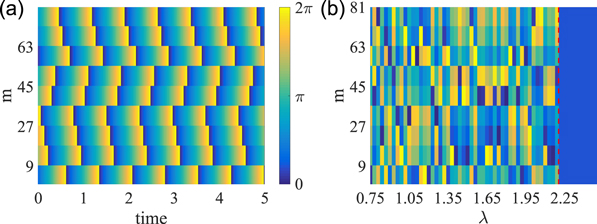
  as shown in figure 6(b).
Figure 6. Cluster synchronized state which is constructed from two factor graphs of an incoherent G1 and a coherent G2. (a) Temporal phase profile for coupling strength λ = 1.35. (b) Snapshot of instantaneous phases for the coupling interval  . The critical coupling of
  is highlighted by the vertical dashed line.
Download figure:
Standard image High-resolution image
If the coupling strength is in a regime that G1 is synchronized while G2 is not, we obtain an N2 clustered synchronization state. Again for illustration purpose, we relabel the oscillators as ![$n=\{[(k-1){N}_{1}+i{]}_{i=1}^{{N}_{1}}\}{}_{k=1}^{{N}_{2}}$](https://content.cld.iop.org/journals/1367-2630/21/12/123019/revision2/njpab5cc7ieqn253.gif) which helps to visualize the Cartesian product operation in the following. On the product model, the phase differences between the kth oscillator
which helps to visualize the Cartesian product operation in the following. On the product model, the phase differences between the kth oscillator  on G2 and all other oscillators
  on G1 are constants, forming one clustered state. Therefore, N2 asynchronous phase oscillators yield N2 clustered synchronization states on the product model.
5. Discussion
In summary, we have provided the WS ansatz to the lower dimensional dynamic equations which describe the high dimensional Cartesian product model that is reconstructed from two independent Kuramoto models on star subgraphs of G1 and G2 by graph operation. The order parameters describing different synchronization states of the product model are expressed by fixed points of the lower dimensional equations. Furthermore, the steady states of the order parameter Z and their respective stabilities have been delineated theoretically. Our numerical simulations agree very well with the theoretical results.
In the case of a single star graph, there is only one discontinuous explosive transition to synchronization in the forward process. In contrast, two explosive jumps in the forward curve have been observed in the product model. The first jump corresponds to a local scale of synchronization of one subgraph only while the other subgraph is not synchronized. The second jump is for the global synchronization for both subgraphs. Between these two jumps, cluster synchronized behavior has been widely obtained, which provides complementary insights for the understanding of cluster synchronization. In the literature, many versions of cluster synchronization scenarios have been reported in various settings, for instance, for unidirectional coupling, time delays and some special network structures [41, 42]. Some numerical algorithms are required to identify synchronized clusters [43] or using graph partitions [44]. Recently, computational group theory has been proposed to characterize cluster synchronization, which hinges on the decomposition of the networked nodes into clusters with the help of network symmetries [25, 26].
In contrast to the literature, cluster synchronized states in this work are reconstructed by the Cartesian product operation which is performed from two independent star networks of phase oscillators. In the product model  , the clustered states are widely observed, especially in the coupling regimes where one factor graph is synchronized while the other factor graph is not. Note that such clustered states are realized for the case that both G1 and G2 are in a forward continuation transition processes (or both are on the backward processes). Furthermore, the linear stability analysis of fixed points identifies further cluster synchronized states that are realized by the Cartesian product of the forward transition process of G1 and the backward process of G2 (or the vise versa). We emphasize that the cluster synchronization solutions are synthetic states which are obtained by graph product operations. Furthermore, we easily get the number of clusters which is determined by the number of asynchronous oscillators of one factor graphs. As it has been demonstrated in [26], there are six symmetries in a star of identical oscillators. One interesting but maybe challenging task is to study how these group symmetries change when performing Cartesian operations from two subgraphs of stars.
In our earlier work of the Cartesian product model on a star and a ring subgraphs [24] (e.g. G1 is a star and G2 is a ring), we focused on disclosing a hybrid state of an explosive forward synchronization transition and a continuous backward desynchronization transition. Furthermore, the critical coupling thresholds for synchronization transitions are obtained by the necessary conditions of synchronized solutions in the linearized equations. In contrast, the WS method provides lower dimensional nonlinear equations for the ensemble order parameter Z. However, in the product of a star and a ring subgraphs, the WS dimension reduction technique can not be applied straightforwardly since the complex common driving force of equation (11) can not be written down explicitly. Therefore, it remains to be challenging to obtain lower dimensional equations for such a case of Cartesian product of arbitrary subgraph structures.
The Cartesian product of graphs is a commutative, associative binary operation on graphs [21] and most of properties can be derived from the factors. Furthermore, in this work a single star graph is modeled by a population of identical units when introducing the phase difference between the hub and leaf nodes. Therefore, dimension reduction techniques like WS and OA can be applied straightforwardly. The Cartesian product model of two star graphs provides an easy way to build a big graph of the Kuramoto phase dynamics. The product operation can be further performed recursively for G1 and G2 or based on more than two subgraphs (i.e. Gn, n ≥ 3), which is one of the interesting topics for future work. In such cases, we expect that cluster synchronized states on the product can be easily constructed since more combinations of synchronization and desynchronization transition processes of subgraphs are involved. Therefore, graph product operations provide a 'bottom-up' framework which may generate much complicate dynamics that are observed in complex systems.
Acknowledgments
Parts of this work have been financially supported by the National Natural Science Foundation of China (Grant Nos. 11872182, 11875132, and 11835003) and the Natural Science Foundation of Shanghai (Grant Nos. 17ZR1444800 and 18ZR1411800).
: Appendix. Möbius transformations
All Möbius transformations are provided below that are necessary for equations (13), (14)


Note that the variables of ξi,k are constants. In addition, in the case of uniform distribution of ξi,k, the global variables α1,2 and ξi,k do not enter the equation for z1,2 and Z [16, 17]. Using these transformations, we can obtain the equation (16) by equalizing the non-exponential terms of the two sides of the equations (13), (14). More specifically, the non-exponential term of the left-hand side of equation (13) reads

and, respectively, that of the right-hand side of equation (14) is

By equalizing the above two terms, we obtain
