


Abstract
We present a study of the magnetic configuration due to step-induced magnetic frustration at ferromagnetic/antiferromagnetic (FM/AFM) interfaces. At a substrate monatomic step edge, a 180° domain wall emerges. A physically appealing form for the thickness dependence of the domain wall width is obtained. It follows a universal behaviour in the whole thickness range, from ultrathin film to bulk and in both cases of an AFM domain wall on top of the FM layer and a FM domain wall on top of an AFM substrate. In the ultrathin limit of the capping layer, the domain wall grows linearly with the slope depending only on the ratio of the inter-layer and intra-layer Heisenberg exchange constants, regardless of the presence of magneto-crystalline anisotropy. These findings are in good agreement with previous experimental observations. As the thickness grows beyond the ultrathin regime, the corresponding thickness dependence departs from linearity and tends to its bulk value. The analytical insights are supported by conclusive numerical simulations of two independent varieties, namely, the Monte Carlo method which also includes the growth kinetics and the object oriented micromagnetic framework based micromagnetic simulations. While the quantitative details of the study are naturally dependent on the specific material parameters of the complex magnetic system, the global features of the spin texture in the capping layer are dictated by the topological step-edge defect. The latter in itself is quantifiable by a winding number of 
Export citation and abstract BibTeX RIS

Original content from this work may be used under the terms of the Creative Commons Attribution 3.0 licence. Any further distribution of this work must maintain attribution to the author(s) and the title of the work, journal citation and DOI.
1. Introduction
One of the most ubiquitous structural defects that accompany the crystal growth of a thin antiferromagnetic (AFM) film on top of a ferromagnetic (FM) substrate, or vice versa, is the monatomic step edge. Indeed, surface defects of this type are practically unavoidable. Their presence at magnetically active interfaces often leads to non-negligible magnetic frustration, resulting in complex spin textures [1–9]. This is especially true for most of the cases of practical relevance, where the exchange coupling across the AFM/FM interface is quite strong and is of primary importance for the understanding and design of various front-edge applications, such as magnetic storage, magnetic sensors, etc [10–12]. Despite its immediate relevance, a comprehensive picture of its emergence and strength remains debatable and is very much a work in progress [3, 13–16]. This is due without a doubt to the complex geometrical and physical nature of the interfaces as well as to the great difficulty of extracting direct experimental information from the buried interfaces and their defects [17, 18]. In particular, magnetic frustration was successfully observed in the Mn/Fe(001) system via spin-polarized scanning tunnelling microscopy (SP-STM) by Schlickum et al [4–6]. In that system, the width of the AFM domain wall (DW) was found to increase linearly as a function of Mn thickness. In an independent study, Yamada et al repeated the same measurement on a system with Mn on top of Fe(001), but found the domain-wall width to be nearly independent of the Mn thickness [19]. Similar frustrated spin configurations have also been reported in other systems [8, 9, 20–30]. The frustration induced domain wall in nanorings is considered to lead to potential logic and memory applications [31].
Here, we report on a theoretical study of magnetic frustrations induced by a monatomic step at an AFM/FM interface. The system initially consists of a hybrid structure with a thin AFM film on top of a FM substrate. To capture the essential physics with a minimum of complicating detail, both film and substrate are assumed to be simple cubic (SC) in structure (figure 1(a)). The analysis can also be extended to body-centered-cubic (bcc) and face-centered-cubic (fcc) structures with essentially the same results. At its core, the model is one of interacting classical spins on a cubic lattice. The monatomic edge step is assumed to be straight and along one of the main cubic-lattice directions (to be labelled as the y-axis), which allows for a further major reduction. Namely, we assume that the spin texture does not change in the y-direction, so that the model of relevance is a two-dimensional one, in which we allow for exchange interaction and magneto-crystalline anisotropy and discard the dipolar contribution. Our analysis shows that the AFM domain-wall width increases linearly with the thickness of the AFM layer in the ultrathin limit, in good agreement with previous experimental findings. With further increase of the thickness of the AFM layer, the dependence deviates from linear with the thickness eventually saturating to its bulk domain wall value. Interestingly, we find that the overall thickness dependence can be described quite well by a universal formula for both two-fold and four-fold symmetry of the anisotropy. Moreover, we also provide a rigorous argument that similar thickness dependence is to be expected for a FM domain wall on top of an AFM substrate. As will be discussed below, the distributions of the magnetization orientation in both cases obey the same equation under a certain transformation. Qualitatively, this can be understood from a topological point of view of the emerging spin texture. In both cases of either an AFM film on a FM substrate or a FM film on an AFM substrate, the monatomic step edge leads to a topological defect in the magnetic structure with an identical winding number of  for both cases [32]. Under the same boundary conditions and the same topological defect at the interface, the domain wall width follows the same capping-layer thickness dependence. Our results are further confirmed by conclusive simulations of two independent varieties, namely, the Monte Carlo method which also includes the growth kinetics and the object oriented micromagnetic framework (OOMMF) based micromagnetic simulations [33].

Figure 1. Sketch of the spin distribution of (a) frustrated AFM on FM substrate (b) frustrated FM on AFM substrate. Spins are all assumed to lie within the (x–z)-plane. Black arrows represent the spin orientation of substrate Q atoms and blue/red/green arrows represent those of P atoms. Red line represents the domain wall boundary and purple line separates P/Q atoms.
Download figure:
Standard image High-resolution image2. General features and topological aspects
Figures 1(a) and (b) present the sketched magnetic configurations of the frustration near a monatomic step edge at an AFM/FM interface. Due to the presence of the step edge, the magnetic structure of the capping layer at the same height on both sides are shifted by one monolayer. Namely, the odd layers on one side are aligned with the even layers on the other side. Since the exchange coupling between the AFM and FM at the interface is the same on both sides of the step edge, the magnetic moments of the film at the same height on both sides are aligned oppositely due to their different 'parity' in thickness as measured by the number of monolayers from the interface. This is in conflict with the intra-layer FM coupling in any given layer, which prefers the magnetic moments to be aligned in the same direction. As a result, a narrow, frustrated region emerges. For an AFM film deposited on a FM substrate, this is the region that we refer to as the AFM domain wall (figure 1(a)). Similarly, a FM domain wall appears when a FM film is deposited on top of an AFM substrate with a monatomic step edge (figure 1(b)). Such spin textures (spin defects) are often pinned at structural defects, such as the monatomic step here, due to the strong interface exchange coupling. It is important to keep in mind that the topological defect one gets to deal with is due to both the structural defect and the magnetic interactions. This would become quite obvious, also in its details, in what follows.
In systems with strong/dominant exchange coupling across the interface, the frustrated spin texture is pinned at the structural defect (the monatomic step). Thus, we find ourselves in the archetypal situation of a non-uniform magnetic medium, where the magnetization (the order parameter) varies continuously through space except at isolated regions of lower dimensionality [34]. In principle, the structural defect could be a topological defect all by itself if one is concerned with, say, the strain field that it directly relates to. However, it is the combination of the structural defect with the competing AFM and FM exchange interactions at the interface, and especially at the location of the defect, that gives rise to the magnetic topological defect and the related frustrated spin texture, which are of interest here.
The magnetic topological defect is much stronger than a mere discontinuity in the order-parameter field. Indeed, the spin distribution is substantially singular and increasingly dominated by the exchange interaction as one approaches the low-dimensional manifold of the step-edge defect. The peculiarity of such a situation was first realized and described by Feldtkeller for the case of a Bloch point in a micromagnetic domain structure [35, 36]. Early on, Doering exposed the micromagnetic singular-point problem in all clarity and added much to its quantitative understanding [37].
One can now capture the topological aspect 'at closer range' by estimating the winding number of the domain walls shown in figures 1(a) and (b). The step edge can be viewed as a knot due to the magnetic singularity. The magnetic moment near the interface in the capping layer rotate their magnetization by 180° across the step edge. This is analogous to the topological domain walls with the winding number of  mentioned by Tchernyshyov and Chern [32]. The only difference is that the domain wall considered in [32] occurs at the boundary of a finite FM while the domain walls, discussed here, emerge at the FM/AFM interface. However, since the spins in the substrate and just below the interface are aligned collinearly, they have zero contribution to the winding number (see also the part, devoted to the planar ferromagnet in the paper by Mermin [34]). Thus, the winding number remains unchanged regardless of whether there is a substrate or not. Therefore, from the topological point of view, the domain walls discussed here are identical with the FM domain walls discussed in [32], except that here we consider both AFM and FM domain walls.
3. The analytical model and results
Figure 1(a) depicts schematically the anticipated texture for an uncompensated layered-AFM frustration of an AFM/FM bilayer system. The magnetic moments are assumed to align within the (x–z)-plane, however, the main conclusions also hold when the moments rotate within the (x–y)-plane only. Atoms in the capping film are labelled as P, while those in the substrate are labelled as Q. As shown by the magnetic configuration, the interlayer/intralayer coupling within P is AFM/FM, respectively. We further assume the interface coupling between P and Q atoms is AFM (we note that the same conclusions can be drawn for the case of FM coupling at the interface). For simplicity, both the in-plane and out-of-plane lattice constants of P are assumed to be equal to those of Q. In reality, there is always a small lattice mismatch due to the hetero-growth [19, 22]. However, its effect on the frustrated structure is weak. Typically, the thickness of P is small compared with the thickness of the Q layer, and the magnetic frustration occurs only in the P film near the substrate step edges as shown in figure 1(a). The situation may become more complicated if both P and Q are ultrathin films. Depending on the relative strength of the coupling P–P, Q–Q, and the coupling P–Q across the interface, frustration may arise in either the AFM or the FM layer [7].
For sufficiently large negative x (far left in figure 1(a)) and large positive x (far right in figure 1(a)), the unperturbed AFM layered structure will persist. Since the strong exchange coupling fixes the spin orientation of the P atoms at the interface, the spins of the P atoms on the two sides of the step edge have nearly opposite orientations. Thus, frustration is bound to set in within a finite length near the monatomic step-edge defect. The relatively narrow region of frustrated spin texture between the large regions of undisturbed AFM ordering is a domain wall [38, 39]. Clearly, one anticipates that here the DW width is P-layer dependent. Previous experimental work established that the DW width, which we choose to denote as  for the Mn/Fe(001) system is proportional to the thickness d of the P-atomic layers, that is,
  [4]. This is equivalent to say that the angle between DW boundary curve (red line in figure 1(a)) and the x-axis is about 45°.
Altogether, we are led to consider the following model, which will prove sufficient to capture the salient features of the experimental and qualitative observations described above. In essence, the system can be approached as a layered two-dimensional antiferromagnet of classical spins with nearest-neighbour exchange interactions and with cubic or uniaxial magneto-crystalline anisotropy. The system interacts strongly and antiferromagnetically with the hard ferromagnetic substrate across the interface (purple line in the x–z plane in figure 1(a)), so that the spins in the lowermost AFM layer are antiferromagnetically pinned to the topmost substrate layer. The latter assumption enforces the topological magnetic defect, discussed above; it also makes possible a weaker, 'local' effect, namely, the possibility for uniaxial magneto-crystalline anisotropy in an otherwise cubic-symmetry system. The dipolar interaction between the spins will not be included in the model. It has been considered in other, quite distinct (magnetically very soft) systems, where magneto-crystalline anisotropy in the frustrated system has been ignored and the so-called micromagnetic limit has been assumed [32, 40–42]. There, the micromagnetic pole-avoidance principle for bulk and boundary alike has been implemented in order to argue for the pinning of the spin structure at a point at the interface of a two-dimensional system. In a well-defined sense, the magnetic topological defect in these studies and other systems results from the dressing of the boundary point defect by different dominant physical circumstances.
Within the specified model, the competing interactions that will determine the spin texture (including the DW width) are the intralayer exchange coupling, the interlayer coupling, and the topological defect, arising from the dressing of the 'bare' structural defect with the strong exchange interaction across the interface. In principle, at this point one could resort to a Landau–Bloch–Kittel micromagnetic description [39, 43–45] except that there is a steep hurdle in the way: due to the layered AFM structure of the capping film, the directions of the magnetic moments of adjacent P layers are almost opposite (indeed, the adjacent-layer spins are nearly maximally misaligned). This nearly perfect discontinuity makes it impossible to pursue the integration for the total magnetic energy. To circumvent this difficulty, we have devised a transformation for the magnetic configuration  where
where  is the angle between the orientation of the local moment at the site
  with respect to the positive x axis, and i and j represent the x-coordinate and the z-coordinate of the atoms, respectively, with
  being integers. Now, a new, conjugate spin distribution function
  is introduced where spins in odd layers have the same orientation as those in the configuration of interest
  while spins in even layers have the opposite orientation to those in
  The effect of this transformation is that all magnetic moments in the even layers are rotated by 180° with respect to their original orientations. The mathematical form of the transformation can be given as:

With this transformation, the FM system and AFM system are interchanged and the frustrated AFM system in figure 1(a) converts to the frustrated FM system shown in figure 1(b).
In the frustrated ferromagnetic system, both the intralayer coupling  and interlayer coupling
  are positive, i.e. of ferromagnetic type. In the antiferromagnetic system, the intralayer exchange coupling is ferromagnetic (
 ) while the interlayer exchange coupling is antiferromagnetic (
 ). The central point of introducing the conjugate system is that the frustrated antiferromagnetic system in figure 1(a) has equal energy with the frustrated ferromagnetic system in figure 1(b) under the assumptions spelled out earlier. In other words,
  as is demonstrated in appendix. If
  minimizes
  then
then  minimizes
  The magnetic configuration of AFM can then be obtained by performing an inverse transformation, and the DW boundaries of both systems are the same. The above procedure resolves the discontinuity obstacle and makes it possible to proceed with the implementation of the well-known procedure for continuous modelling of a discrete-spin system and the subsequent variational minimization of the total magnetic energy to the end of determining the spin texture [36, 43–45].
3.1. Two-fold magnetic anisotropy case
We first consider the system having two-fold anisotropy with the anisotropy constant of  After the above-mentioned transformation, the magnetic configuration in P changes from antiferromagnetic to ferromagnetic, and the magnetization varies continuously along the vertical (z) direction. Taking into account the nearest-neighbour exchange interaction in the Heisenberg form
  as well as the magnetic anisotropy energy, the total energy of the system can be obtained as:

Without loss of generality, we set the local spin  and the lattice constant
  in equation (2). The usual variational method for the minimization of the total energy leads to:

which can be cast into the following dimensionless form by simple rescaling with  and
and 

Here,  One should notice that
 and
and  appear only in a reduced form as
  and
and  Obviously, the ratios
  and
and  control the x- and z-axis linear transformations, respectively. Once the spin distribution function with a given set of material parameters
  is obtained, the spin distribution function for any other set
  can be obtained via the linear transformation according to their respective ratios.
In general, equation (4) is a nonlinear partial differential equation of second order in two spatial variables. In particular, it happens to be the elliptical sine-Gordon equation in (2 + 0) dimensions. It has been used previously in the micromagnetic context of describing the magnetic domain walls in ferromagnetic nano-stripes [41, 42]. The equation is a natural generalization of the ordinary nonlinear differential equation that emerges from the variational minimization of the well-known cases of the one-dimensional Bloch and Neel walls, that equation itself being mathematically identical with the nonlinear equation of motion of the pendulum [46]. The respective solutions for the one-dimensional domain-wall case look like a kink, which is steep and narrow for large magneto-crystalline anisotropy so much so that such walls are often considered as infinitely thin, yet carrying a finite amount of domain-wall energy per unit area (see, e.g. [47]). The kink-like aspect suggests that one-dimensional domain walls are essentially spatial (or static/frozen) 'solitons' [48]6 .
It is only natural that the soliton formalism is gaining ground for the (2 + 0) case of micromagnetic import. Thus, the elliptical sine-Gordon equation (4) is known to admit of 2N multiple-soliton solutions with N corresponding to the number of emerging domain walls. The sketch of the two-soliton solution (a single domain wall) is as given in figure 1(a). It is of topological nature and is characterized by a winding number of  Not unexpectedly, this solution, corresponding to the winding numbers of
  is of lowest energy in comparison with the soliton solutions of higher multiplicity for the given boundary conditions [32, 40]. Strictly speaking, the variational equation is an extremal equation, whereby the nature of the extremal function (minimal or maximal) has itself to be explored by investigating the convexity of the energy functional (here:
 ![$E[\varphi (x,z)]$](https://content.cld.iop.org/journals/1367-2630/21/12/123045/revision2/njpab5cbdieqn42.gif) ). The partial differential equations that need to be considered in the process are much more convoluted than the extremising equation itself. The convexity analysis is essentially insurmountable for any nontrivial problem and is hardly ever attempted. Here, in the matter of the lowest-lying solution being the two-soliton one, we rely on one hand on the findings of Tchernyshyov and Chern [32, 40] and Janutka and Gawronski [37, 38] and, on the other hand and even more importantly, on the direct computation by two different methods of the spin configuration, towards which the magnetization relaxes. As will be seen below, a direct Monte Carlo simulation and an independent micromagnetic simulation with the OOMMF code indicate that the spin texture of minimal energy is the domain wall of winding number of
). The partial differential equations that need to be considered in the process are much more convoluted than the extremising equation itself. The convexity analysis is essentially insurmountable for any nontrivial problem and is hardly ever attempted. Here, in the matter of the lowest-lying solution being the two-soliton one, we rely on one hand on the findings of Tchernyshyov and Chern [32, 40] and Janutka and Gawronski [37, 38] and, on the other hand and even more importantly, on the direct computation by two different methods of the spin configuration, towards which the magnetization relaxes. As will be seen below, a direct Monte Carlo simulation and an independent micromagnetic simulation with the OOMMF code indicate that the spin texture of minimal energy is the domain wall of winding number of 
To get an analytical grip on equation (4), we assume that the spin arrangement in the frustrated region follows the known one-dimensional 'kink' profile ![${m}_{x}/{m}_{s}=\,\cos [\varphi (x,z)]=\,\tanh [x/\omega (z)]$](https://content.cld.iop.org/journals/1367-2630/21/12/123045/revision2/njpab5cbdieqn44.gif) for a given z, that is, at a fixed distance from the interface. In it,
for a given z, that is, at a fixed distance from the interface. In it,  is the domain-wall width
  in the z-layer. On one hand, the assumption conforms with experimental observations [4–6], while on the other hand it will turn out to be consistent with direct numerical calculations (see below). When
  the DW is expected to cross over into a bulk domain wall which has the known form of
  When
When  the DW is very narrow as also observed experimentally. Given these boundary conditions in z, a self-suggesting approximate solution for equation (4) can be written down in the form:

with two parameters to be determined,  and
and  By comparing it with the bulk domain wall profile
  with
with  it follows that
  By comparing equation (5) with the one-dimensional domain-wall profile mentioned above, one can obtain the expression for the width as

In the ultrathin limit 
 That is to say, the domain-wall width has a linear dependence on the thickness z, in good agreement with reliable experimental findings [4]. For
  the domain wall is very narrow. In the immediate vicinity of the singular point (
 ), the exchange energy is dominant, and the magnetic anisotropy energy epitomized by the constant
  can be neglected [37]. The sine-Gordon equation then goes into the two-dimensional Laplace equation with specified boundary conditions. By solving the Laplace equation, we obtain
  The solution is a tour de force that culminates in taking the limit of interest, (
 ). It will be reported in detail elsewhere because of its independent interest [49]. Here, we provide heuristic argument as a shortcut to estimate (correctly!) the value of
  Namely, from equation (5), it can be derived that
  at the domain wall boundary position where
  As the domain wall width shows a linear dependence with z at ultrathin limit, it can be anticipat ed that the magnetic moment at the domain wall boundary position to be aligned with the geometrical angle in dimensionless coordinates, so that
  Thus, the value of
  can be obtained as
 ![$\cot \left[\arccos \left(\tan {\rm{h}}\left(1\right)\right)\right]=\,\sin {\rm{h}}(1)\approx 1.175$](https://content.cld.iop.org/journals/1367-2630/21/12/123045/revision2/njpab5cbdieqn67.gif) .
.
With this, one can proceed to obtain the slope of the domain wall width versus the thickness z in the ultrathin limit as:

Evidently, the slope depends only on the ratio of the intralayer and interlayer exchange constants, and is independent of the magnetic anisotropy constant. By assuming  for the Mn/Fe(001) system, the estimated slope is in close agreement with the experimental finding, where a value of 2.24 was derived from [4].
As mentioned above, the determination of the initial slope is based on the rigorous asymptotics of the Laplace-equation solution close to the singularity, which is at the origin in figure 2. The formula (7) can equivalently be seen as providing a way to estimate the ratio of the exchange constants if the experimental initial slope has been determined reliably. Thus, applying this procedure to the findings of Schlickum et al [4], denoting the experimental slope as  and inserting it into the left hand side of equation (7), one finds
 ![${J}_{s}/{J}_{d}={[{S}_{{\rm{e}}{\rm{x}}}/2\sin {\rm{h}}\left(1\right)]}^{{\rm{2}}}=0{\rm{.91}}$](https://content.cld.iop.org/journals/1367-2630/21/12/123045/revision2/njpab5cbdieqn70.gif) where the value of
where the value of  has been taken from [4]. Therefore, the theory developed here offers access to microscopic exchange parameters, which have traditionally been notoriously difficult to extract from experiment.

Figure 2. (Wide) Spin distribution obtained with Monte Carlo simulations for systems with two-fold magnetic anisotropy. (a) ∼0.3 ML AFM grown on FM, (b) ∼8.5 ML AFM grown on FM, (c) ∼0.3 ML FM grown on AFM, and (d) ∼8.5 ML FM grown on AFM. Colour wheel shows the relation between colour and spin orientation. Purple line marks the FM/AFM interface.
Download figure:
Standard image High-resolution imageIn writing down the model (2), we used exchange-integral ( ) notation for the already coarse-grained, continuous, micromagnetic functional. The intention was to allow for a better understanding of the conjugation transformation, which makes possible the continuum modelling of the antiferromagnetic domain wall. One can now return to the established micromagnetic notations, involving the exchange stiffness A. In doing this, we summarize the salient features of the proposed approximate solution, while at the same time we extend the SC symmetry findings to the cases of bcc and fcc symmetry


3.2. Four-fold magnetic anisotropy case
Above, we discussed the case of two-fold magnetic anisotropy. In the following, we examine the case of four-fold magnetic anisotropy. In this case, too, due to the strong pinning at the interface  domain walls are formed. This will be also confirmed by the numerical simulations below. Thus, we focus our discussion on the case of a
  domain wall. With the magnetic anisotropy of
  and using the variational method as before, one can easily derive the condition for the stable magnetic configuration as:

Through a linear rescaling of 
 and
and  equation (8) can be cast as a dimensionless one similar to equation (4), namely,

The only difference is that  changes from 0 to
  (while
  varied from 0 to
  ) when
  changes from
  to
to  Following the procedure discussed above, one finds that the thickness-dependent domain-wall profile and domain-wall width can be described by expressions, similar to the two-fold ones:


with  and
and  Interestingly, at the ultrathin limit, the domain wall width is the same for both two-fold and four-fold anisotropy cases,
  This again proves that the domain wall width at the ultrathin limit is independent of the strength and type of magneto-crystalline anisotropy.
4. Micromagnetic simulations
Here, the Monte Carlo method is employed to simulate the magnetic moment relaxation during the growth process. The magnetic orientation of each moment at the cross section of the frustrated region (figure 1(a)) can be described by a two-dimensional matrix ![$\varphi \left[i\right]\left[j\right],$](https://content.cld.iop.org/journals/1367-2630/21/12/123045/revision2/njpab5cbdieqn93.gif) where
where  and
and  denote the x- and z-coordinates. Each element in the matrix represents the spin orientation of one atom. The initial state is the Q-atomic substrate only. With time, P atoms are deposited randomly onto the substrate at a certain rate, which is low enough for P adatoms to reach their magnetic equilibrium state. For simplicity, an atom is assumed to be anchored once it is deposited, which is to say that surface diffusion of the deposited atoms is forbidden. After a P-atom is deposited, its spin orientation is allowed to remain unchanged or to be tilted by a small angle positively or negatively within the (x–z)-plane. Thus,
 ![$\varphi \left[i\right]\left[j\right]$](https://content.cld.iop.org/journals/1367-2630/21/12/123045/revision2/njpab5cbdieqn96.gif) becomes
becomes ![$\varphi \left[i\right]\left[j\right]+{L}_{n}$](https://content.cld.iop.org/journals/1367-2630/21/12/123045/revision2/njpab5cbdieqn97.gif) with a characteristic change of energy:
with a characteristic change of energy:  where L0 = 0, L1 = ∆L, L2 = −∆L, respectively. The P-atom is switched to the state with minimal energy. The size of ∆L is gradually decreased from 0.01 to 0.0001, so that one can drive all elements in the matrix
 ![$\varphi \left[i\right]\left[j\right]$](https://content.cld.iop.org/journals/1367-2630/21/12/123045/revision2/njpab5cbdieqn99.gif) to relax into their global minimal energy states with sufficiently high precision within a reasonable simulation period. The whole procedure is repeated every time a new P-atom is deposited, making sure that the system is always in its minimal energy state. The simulations stop when the desired thickness of the P layer is reached with the system relaxed into its most stable state.
to relax into their global minimal energy states with sufficiently high precision within a reasonable simulation period. The whole procedure is repeated every time a new P-atom is deposited, making sure that the system is always in its minimal energy state. The simulations stop when the desired thickness of the P layer is reached with the system relaxed into its most stable state.
4.1. Two-fold magnetic anisotropy case
Figures 2(a) and (b) present two snapshots of the growth process of an AFM layer with two-fold anisotropy on a FM substrate. The colour wheel defines the relation between colour and spin orientation. The thin purple line marks the FM/AFM interface. Figure 2(a) shows a typical magnetic configuration at the initiation of the growth process, i.e. at about 0.3 ML. The spin orientations of substrate FM atoms lie along the x-direction. Due to the strong AFM exchange coupling between the AFM and FM layer, the spin orientation of AFM atoms at the interface is antiparallel to that of FM atoms. With increasing the AFM thickness, a frustrated region forms near the step edge. At a thickness of about 8.5 MLs of AFM atoms, the system relaxes into the state, shown in figure 2(b). In each AFM layer, the spin orientation changes with respect to that layer's midpoint above the step edge by 180° over a narrow range, whereby the domain wall widens with the increase of the AFM thickness. In the simulation, the exchange constant of the FM atoms is assumed to be much larger than that of the AFM atoms. Thus, magnetic frustration only appears in the AFM layer. Figures 2(c) and (d) present the simulated results for a FM film deposited on an AFM substrate at the initial and final growth stages, respectively. In this case, magnetic frustration occurs in the FM layer while the DW width again increases with the increase of the FM layer thickness. The complete growth process can be monitored in the supplementary movies (SM1 and SM2) is available online at stacks.iop.org/NJP/21/123045/mmedia.
Figure 3 illustrates the simulated position-dependent magnetic moment orientation of the representative layers from 1 ML to 40 MLs for both the AFM grown on FM and the FM grown on top of an AFM substrate for the two-fold anisotropy case. The red/blue symbols represent the simulated results for AFM grown on FM and FM grown on AFM substrate, respectively. The black lines represent the one-dimensional domain-wall profile, determined in the analytical part of this study. Clearly, the magnetic orientation in each layer is described rather well by the 1D DW formula, validating the approximation adopted in the analytical calculation. The simulated results for both cases are almost identical. Also, the domain-wall width increases with the thickness in qualitative agreement with the analytical calculation and the experimental findings.
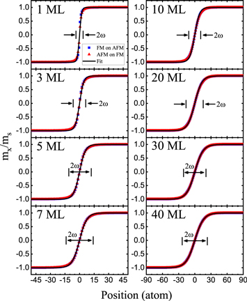
Figure 3. Simulated layer dependent domain wall profile for two-fold anisotropy case with the layer thickness marked in each panel. Red and blue symbols are simulated results for AFM grown on FM and FM grown on AFM, respectively. The black lines are the fitting using the 1D domain wall profile. Detailed parameters used in the simulations are: 
 and
and 
Download figure:
Standard image High-resolution imageTo zoom into the quantitative information in greater detail, we plot the domain-wall boundary in figure 4(a) and the domain-wall width in figure 4(b) as functions of the thickness for various values of 
 and
and  Normalized units of
  and
and  are used along both the x- and the z-axis. For comparison, we also plot the result obtained by the analytical method (black curve). All domain-wall boundaries for systems with different parameters collapse onto a single curve under the linear rescaling transformation. The Monte Carlo simulations also agree well with the analytical solution in equation (5). The slight deviation originates in the finite thickness that has to be used in the simulations. When the thickness of the top layer is increased, the agreement between simulation and analytical calculation is improved. Therefore, the spin conjugation transformation allowing for a continuous description of the AFM domain wall, the spin distribution formula given in equation (5), and the initial-slope relation of equation (7) are all confirmed by the Monte Carlo simulations.
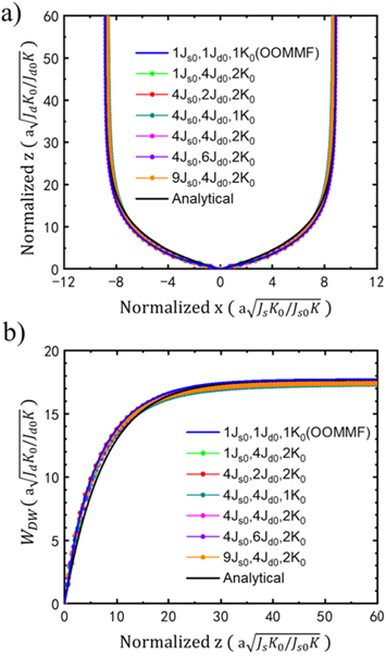
Figure 4. Thickness-dependent domain-wall boundary (a) and domain-wall width (b) obtained with Monte Carlo simulations for two-fold anisotropy and with different sets of values  The specific values for the material parameters are

 The results of the analytical calculation and the micromagnetic simulation with OOMMF code are also plotted for comparison.
Download figure:
Standard image High-resolution imageWe also performed micromagnetic simulations using the OOMMF code. Because OOMMF cannot simulate the magnetic structure of AFM materials except down to atomic level, we study only the frustration in a FM layer on top of an AFM substrate. The uppermost layer of the AFM substrate is fixed. The results from OOMMF are represented in figure 4 by the blue curves. They are consistent with the analytical calculations and the Monte Carlo simulations.
4.2. Four-fold magnetic anisotropy case
We performed analogous simulations for the four-fold magnetic anisotropy case. Interestingly, we found that there is only a  domain wall forming near the step edge in spite of the four-fold nature of the magnetic anisotropy. This could be understood as follows. At the interface, the exchange energy is dominant as compared with the magnetic anisotropy energy. The geometrical constraint requires the magnetization of the film to be collinear with the substrate magnetization, independently of whether the coupling at the interface is ferromagnetic or antiferromagnetic. On both sides of the step edge, the orientation of the substrate magnetization is also collinear. Such requirements essentially result in strong effective two-fold magnetic anisotropy. Thus, a
  domain wall is formed. As the film thickness increases, this effective two-fold anisotropy is weaker and the domain wall widens.
Figure 5(a) presents the comparison of the thickness dependent domain wall boundary for two-fold and four-fold magnetic anisotropy cases utilizing the same  and
and  where
where  K0 = 2.56 × 10⁴ J m−3. The symbols correspond to the Monte Carlo simulations while the lines are the analytical results. The simulated results support the analytical ones. The comparison also shows that at a very small thickness (z < 5), the two datasets overlap. Hence, the domain-wall width as well as its initial slope are the same for both two-fold and four-fold magnetic anisotropy cases, once again in accordance with the analytical results. At a higher thickness, the domain-wall width for the four-fold anisotropy case is generally larger than that for the two-fold anisotropy case.

Figure 5. (a) Comparison of the thickness dependent domain wall boundary for two-fold and four-fold magnetic anisotropy cases utilizing the same 
 and
and  (b) Domain wall width obtained with Monte Carlo simulations for four-fold anisotropy case and with different combination of
 and
and  Detailed parameters are


Download figure:
Standard image High-resolution imageFigure 5(b) shows the DW width for the four-fold anisotropy case with different sets of values for the material parameters  We find that at large values of the parameter ratios of
 and
and  the simulated results agree well with the analytical calculations. At small parameter ratios, the simulated results deviate from the analytical ones. The smaller the ratio is, the larger deviation is found. Also, the deviation occurs mainly at higher thicknesses. This can be understood as follows: as mentioned above, the geometrical constraint at the interface can be considered as an effective two-fold magnetic anisotropy. In the ultrathin limit, this two-fold anisotropy is dominant. At a higher thickness, the influence of the interface is weaker; accordingly, the effective two-fold anisotropy is weaker, too, leading to a widening of the domain wall. Even though the nominal anisotropy is four-fold, the admixture of the effective anisotropy from the interface makes the system behave as having mixed two-fold and four-fold anisotropy. In such a case, the domain wall width is larger [32] and deviates from the analytical result: the smaller the ratios of
 and
and  the larger the deviation. Another characteristic behaviour of the domain wall from the combination of the two-fold and four-fold magnetic anisotropy is that the domain-wall profile also deviates from the ideal tanh function [36]. At high thickness and small ratios of
 and
and  this is indeed the behaviour that we observed in simulations.
5. Summary and outlook
We investigated the step-edge induced magnetic frustration at FM/AFM interfaces analytically and by numerical simulations. At substrate monatomic step edges, 180° domain walls of variable width appear, regardless of whether the system possesses two-fold or four-fold magnetic anisotropy. The domain walls are found to be of topological origin and are characterized by a winding number of  In the ultrathin limit, the domain wall width depends linearly on the thickness. The rigorous calculation of the ultrathin limit derives from the general solution of a two-dimensional Laplace equation with appropriate boundary conditions that governs the corresponding system where anisotropy may be neglected. The initial slope depends only on the ratio of the inter- and intra-layer Heisenberg exchange constants, remaining insensitive to the strength and type of magneto-crystalline anisotropy present. Upon increasing the thickness, the dependence deviates from linear behaviour and follows a characteristic exponential form before eventually saturating to its bulk value. For the case of an AFM layer on top of an FM substrate, analytical advance is made possible by employing a novel, ad hoc spin transformation to map the AFM configuration to an FM one with the same energy. The analytical results are further confirmed by numerical simulations by means of the Monte Carlo method and the OOMMF code. The kinetics of the growth process can be monitored in the provided supplementary movies (SM1 and SM2). These findings explain recent experimental observations in such systems in the ultra-thin limit of the capping layer. Notably, they open an independent route, based on the exact results for the initial slope of the topological domain wall, towards the identification of the microscopic exchange parameters in the systems involved.
An exciting path for the implementation of our analysis lies in its applicability to ferroelectric systems where frustration induced domain walls have also been observed and where the domain wall width has been found to increase with thickness at ultrathin region [51]. In both the ferromagnetic and the ferroelectric applications, one can proceed to consider the effect of overlapping domain walls when the step edge defects may interfere. Yet another intriguing possibility is to investigate experimentally suitable systems with a ferromagnetic capping layer on top of an AFM.
In the above, we discussed various cases for spins, restricted in their rotations within (x–z)-plane. We also performed the calculations for the case of spins, lying within the (x–y)-plane and found that both cases lead to essentially the same conclusions. Moreover, if the anisotropy energy term takes a general form ![$U[\varphi (x,z)]$](https://content.cld.iop.org/journals/1367-2630/21/12/123045/revision2/njpab5cbdieqn137.gif) instead of the pure two-fold or four-fold ones that we discussed above, similar analysis applies. The domain-wall width in the ultrathin limit and its initial slope will be the same and dictated by equation (7), since they are independent of the magnetic anisotropy. However, in the analytical calculations and the Monte Carlo simulations several effects, such as the intermixing at the interface, the influence of the finite length of the monatomic step, etc., have been neglected. These may cause deviations of the theoretical results from experiments, yet they could be considered within the outlined framework. Nevertheless, qualitative agreement is to be expected as long as the topology and the leading contributions to the energetics are those that have been spelled out in this study.
instead of the pure two-fold or four-fold ones that we discussed above, similar analysis applies. The domain-wall width in the ultrathin limit and its initial slope will be the same and dictated by equation (7), since they are independent of the magnetic anisotropy. However, in the analytical calculations and the Monte Carlo simulations several effects, such as the intermixing at the interface, the influence of the finite length of the monatomic step, etc., have been neglected. These may cause deviations of the theoretical results from experiments, yet they could be considered within the outlined framework. Nevertheless, qualitative agreement is to be expected as long as the topology and the leading contributions to the energetics are those that have been spelled out in this study.
Acknowledgments
This work was supported by the National Key Research & Development Program of China (No. 2018YFA0306004 and 2017YFA0303202), and by the National Natural Science Foundation of China (No. 11974165, 51971110, 11734006 and 11727808). Critical remarks by the anonymous referees that led to the improvement of the paper are gratefully acknowledged.
Appendix
Theorem:
Proof:
We denote the spin distribution in figure 1(a) as  while that in figure 1(b) as
  The most important difference between the two systems is the interlayer exchange coupling constant,
  for the frustrated FM system and
  for the frustrated AFM system. Other parameters are the same, i.e.

The energy of the frustrated FM system can be expressed as:
Now, the energy of the frustrated AFM system can be expressed as:
The final expression above is identical to E_FM(phi), hence, the energy of frustrated AFM system is equal to that of frustrated FM system:  Q.E.D.
Footnotes
- 6
The soliton terminology has pervaded the many applications of the usual, evolution-type, hyperbolic sine-Gordon equation in (1 + 1) dimensions,
![$\tfrac{{\partial }^{2}\varphi \left(x,t\right)}{\partial x\partial t}=\,\sin \left[\varphi \left(x,t\right)\right],$](data:image/png;base64,iVBORw0KGgoAAAANSUhEUgAAAAEAAAABCAQAAAC1HAwCAAAAC0lEQVR42mNkYAAAAAYAAjCB0C8AAAAASUVORK5CYII=) which comes as no surprise, knowing that this latter equation is one of the few first and best studied soliton equations (see [48]). In co-moving coordinates, the equation can be cast as where we used the same letters in the new coordinate system as here we are only interested in the form of the equation, not in its details. Clearly, this is a nonlinear wave equation with a sine nonlinearity. Note that the label 'sine-Gordon equation' has been used also with different trigonometric nonlinear terms, equivalent or generalizing the sine case, in general, (n + 1) number of dimensions, where the singled-out independent variable is time-like.
which comes as no surprise, knowing that this latter equation is one of the few first and best studied soliton equations (see [48]). In co-moving coordinates, the equation can be cast as where we used the same letters in the new coordinate system as here we are only interested in the form of the equation, not in its details. Clearly, this is a nonlinear wave equation with a sine nonlinearity. Note that the label 'sine-Gordon equation' has been used also with different trigonometric nonlinear terms, equivalent or generalizing the sine case, in general, (n + 1) number of dimensions, where the singled-out independent variable is time-like.
![$\tfrac{{\partial }^{2}\varphi \left(x,t\right)}{\partial x\partial t}=\,\sin \left[\varphi \left(x,t\right)\right],$](https://content.cld.iop.org/journals/1367-2630/21/12/123045/revision2/njpab5cbdieqn38.gif)
![$\tfrac{{\partial }^{2}\varphi \left(x,t\right)}{\partial {x}^{2}}-\tfrac{{\partial }^{2}\varphi \left(x,t\right)}{\partial {t}^{2}}=\,\sin \left[\varphi \left(x,t\right)\right],$](https://content.cld.iop.org/journals/1367-2630/21/12/123045/revision2/njpab5cbdieqn39.gif)