Beating the repeaterless bound with adaptive measurement-device-independent quantum key distribution

The schematic layout of the AMDI-QKD protocol [37] can be seen in figure 1. The protocol runs as follows:

• 1.  
  Each of Alice and Bob generates m signals with their on-demand entanglement sources S_AC and S_BC, respectively. One mode of each signal is sent to Charlie's QND measurement simultaneously via the quantum channel, using a multiplexing technique (e.g. wavelength based). The other mode is kept by Alice and Bob and they measure it in the Z or X basis, which they choose with probabilities p_Z and ${p}_{{X}}=1-{p}_{{Z}}$, respectively.
• 2.  
  Charlie applies QND measurements to the incoming pulses to confirm the arrival of the signals coming from Alice and Bob.
• 3.  
  Charlie pairs the successfully arriving signals via optical switches and performs BSMs between signals coming from the different parties. To be more precise, if there are, say n_A (n_B) successfully arriving signals from Alice (Bob), then Charlie performs $\min ({n}_{{\rm{A}}},{n}_{{\rm{B}}})$ BSMs.
• 4.  
  Charlie announces to Alice and Bob which BSMs were successful, together with the measurement result obtained. Here the successful BSM is assumed to distinguish the Bell states $\left|{\psi }^{-}\right\rangle =1/\sqrt{2}(\left|{HV}\right\rangle -\left|{VH}\right\rangle )$ and $\left|{\phi }^{-}\right\rangle =1/\sqrt{2}(\left|{HH}\right\rangle -\left|{VV}\right\rangle )$ from the others, as we consider (see figure 3 in section 3) a standard linear-optics implementation of the BSMs. Here H (V) represents a horizontally (vertically) polarized single-photon state.
• 5.  
  For key generation, Alice and Bob post-select the events by communicating over an authenticated classical channel where they used the Z-basis to measure their modes in step 1 (and in which they both had a successful photon detection) and also the corresponding BSM was successful. To make sure that their key bits are identical, they apply a bit flip procedure [32]. To be precise, Alice or Bob flips her or his bits, except for the cases when they chose the Z basis and Charlie's BSM outcome was the state $\left|{\phi }^{-}\right\rangle =1/\sqrt{2}(\left|{HH}\right\rangle -\left|{VV}\right\rangle )$.

Zoom In Zoom Out Reset image size

The secret key rate formula for the protocol above has been derived in [37] when the number of multiplexing m tends to infinity. It reads:

$$\begin{eqnarray}&&R={p}_{{Z}}^{2}\,{p}_{{\rm{s}}}\,{p}_{\mathrm{BSM}}\,[1-f\,h({e}_{{Z}})-h({e}_{{X}})],\end{eqnarray} \tag{ 1 }$$

where p_s is the probability that Charlie's QND and the Z measurements are both successful either at Alice's or Bob's site. The quantity p_BSM represents the success probability of one BSM. The quantities e_Z and e_X, on the other hand denote the bit and phase error rates, respectively. The parameter f is an inefficiency function for the error correction process and $h(x)=-x{\mathrm{log}}_{2}(x)-(1-x){\mathrm{log}}_{2}(1-x)$ is the binary entropy function. We remark that the fact that in equation (1) only p_s rather than the square of it appears is due to the advantage that the original AMDI-QKD protocol offers, that is, BSMs are only performed between signals that survived the channel loss. Therefore, a particular signal only needs to survive traveling through one path [37].

We also note that since we evaluate the secret key rate in the asymptotic regime where $m\to \infty$, the parties perform steps 1–5 of the protocol only once. Also, for simplicity, we assume that ${p}_{{Z}}\gg {p}_{{X}}$, so that we take ${p}_{{Z}}^{2}\approx 1$ in equation (1) for the simulations below. Moreover, we assume for simplicity that f = 1.

The full-mode analysis of the AMDI-QKD protocol described above can be found in appendix B, based on equation (1) and the device models described in the next section.

We shall assume that all entanglement sources emit states of the following form:

$$\begin{eqnarray}&&\left|\psi \right\rangle =\displaystyle \sum _{n=0}^{\infty }\,\sqrt{{p}_{n}}\,\left|{\phi }_{n}\right\rangle ,\end{eqnarray} \tag{ 2 }$$

where ${\sum }_{n=0}^{\infty }{p}_{n}=1$ and ${p}_{n}\geqslant 0$. The n-photon pair states $\left|{\phi }_{n}\right\rangle$ are given by

$$\begin{eqnarray}&&\left|{\phi }_{n}\right\rangle =\displaystyle \frac{1}{n!\,\sqrt{n+1}}{\left({x}_{H}^{\dagger }{y}_{H}^{\dagger }+{x}_{V}^{\dagger }{y}_{V}^{\dagger }\right)}^{n}\left|0\right\rangle ,\end{eqnarray} \tag{ 3 }$$

where ${x}_{H}^{\dagger }$ and ${y}_{H}^{\dagger }$ (${x}_{V}^{\dagger }$ and ${y}_{V}^{\dagger }$) are the creation operators of horizontally (vertically) polarized photons in the modes x and y, respectively and $\left|0\right\rangle$ denotes the vacuum state.

We note that if we choose p₁ = 1 (i.e. p_n = 0 for any $n\ne 1$) then equation (2) represents a perfect entanglement source that is capable of emitting maximally entangled states $\left|{\phi }_{1}\right\rangle$ with certainty. Another interesting special case is when

$$\begin{eqnarray}&&{p}_{n}=\displaystyle \frac{(n+1){\lambda }^{n}}{{\left(1+\lambda \right)}^{n+2}},\end{eqnarray} \tag{ 4 }$$

holds, in which case equation (2) describes a type-II PDC source [41] with λ being a positive parameter, related to the amplitude of the pumping laser.

We shall assume that all the detectors are PNR detectors, characterized by the following positive operator-valued measure (POVM) elements

$$\begin{eqnarray}&&{{\rm{\Pi }}}_{k}=\displaystyle \sum _{n=k}^{\infty }\displaystyle \left(\genfrac{}{}{0em}{}{n}{k}\right){\eta }_{\det }^{k}{\left(1-{\eta }_{\det }\right)}^{n-k}\left|n\right\rangle \left\langle n\right|,\end{eqnarray} \tag{ 5 }$$

with $k=0,1,\cdots ,\infty$ denoting the number of detected photons. In equation (5), the parameter ${\eta }_{\det }$ is the detection efficiency of the detectors and $\left|n\right\rangle$ is the n-photon Fock state. We note that for simplicity in equation (5) we have disregarded the dark count probability of the PNR detectors.

A linear-optics teleportation-based implementation of the QND measurement can be seen in figure 2. It consists of a standard linear-optics BSM module together with an entanglement source ${S}^{\mathrm{QND}}$ that emits the state described in equation (2). The purpose of the QND measurement module is to herald if a photon successfully arrived at Charlie's node, so that, in this case, he can continue the protocol with performing his BSMs. The successful heralding events are constituted by the same detection patterns as in the original MDI-QKD protocol [32], that is, a successful heralding event occurs if the detectors detect exactly one photon in horizontal polarization and one photon in vertical polarization. The setup is based on quantum teleportation. Indeed, in the case of a single-photon input and S^QND being a perfect EPR source with p₁ = 1, the QND module teleports its input mode to its output mode [42]. We note that there exist more efficient implementations of a BSM [43, 44] in terms of the success probability (which can approach 1 instead of 1/2 as in the scheme shown in figure 2), but they come with the overhead of the need for complicated ancilla states.

Zoom In Zoom Out Reset image size

Charlie directs the successfully arriving signals into his BSMs with the help of optical switches. For this, an active feedforward mechanism is required since it takes time to align the ports of the switches properly, so that successful signals from Alice and Bob end up in the same BSM at Charlie's site. It is assumed that one active feedforward takes time τ, during which signals propagate in optical fibers. Therefore, the feedforward procedure can be modeled as a lossy channel with transmittance ${\eta }_{{\rm{f}}}=\exp (-\tau c/{L}_{\mathrm{att}})$ due to the propagation of the signals through the fibers, where c denotes the speed of light in the optical fiber. Otherwise, we assume perfect switching devices with unlimited number of entries.

In this case, the linear-optics implementation of the middle BSM modules is depicted in figure 3. Similarly to the QND module, the success events are constituted by the same detection patterns as in the original MDI-QKD protocol [32]. Note, however, that this middle BSM module differs from the one used in the QND measurement. Here, Hadamard gates (denoted in figure 3 by H) are applied [39], whose operation can be described as

$$\begin{eqnarray}&&\left[\begin{array}{c}{y}_{H}^{\dagger }\\ {y}_{V}^{\dagger }\end{array}\right]=\displaystyle \frac{1}{\sqrt{2}}\left[\begin{array}{cc}1 & 1\\ 1 & -1\end{array}\right]\left[\begin{array}{c}{x}_{H}^{\dagger }\\ {x}_{V}^{\dagger }\end{array}\right],\end{eqnarray} \tag{ 6 }$$

where ${y}_{H}^{\dagger }$ (${y}_{V}^{\dagger }$) and ${x}_{H}^{\dagger }$ (${x}_{V}^{\dagger }$) are the creation operators of the input and output modes of the Hadamard gate in horizontal (vertical) polarization.

Zoom In Zoom Out Reset image size

Including the Hadamard gates is advantageous, since they can prevent errors that can occur otherwise. For example, when the source S^QND emits a two-photon pair state and the input of the QND module is the vacuum state, a successful heralding event can still occur, despite of the fact that the signal coming from the corresponding party was lost. In this scenario, it can be shown (see appendix A) that the output state of the QND measurement, heading towards the middle BSM, is a two photon signal consisting of one vertically and one horizontally polarized photon. Now, without the Hadamard gates, this state could give a successful detection event at the middle BSM, which is undesired since there was no signal received from the party connected to the seemingly successful QND measurement. Intuitively, one expects that adding the Hadamard gates, i.e. rotating the signal, will just decrease the chance of the two photons ending up in detectors corresponding to different polarizations. This is so because, after the rotation, it is not predetermined any more which detector they hit after the polarizing beam splitter, and it rather becomes a probabilistic process. However, carrying out the calculation shows (see appendix A) that, in fact, the Hadamard gates force the spurious two photon signal to give non-conclusive detection events at the final BSM, which is the best possible scenario. In short, in this example the actual signal from at least one party is lost, and therefore obtaining a conclusive key generation event will essentially introduce an error with probability 1/2 due to the fact that the parties do not share the desired quantum correlation since their emitted signals have not actually interacted. Consequently, it is advantageous for Alice and Bob to reflect such an event as a non-conclusive event of the protocol with the help of the Hadamard gates, instead of getting a conclusive one which will introduce an error with high probability.

For concreteness, we assume that the quantum channel connecting Alice (Bob) to Charlie is an optical fiber with attenuation length L_att and transmittance

$$\begin{eqnarray}&&{\eta }_{\mathrm{ch}}=\exp \left[-\displaystyle \frac{L}{2{L}_{\mathrm{att}}}\right],\end{eqnarray} \tag{ 7 }$$

where L is the distance between Alice and Bob, and ${L}_{\mathrm{att}}=10\,{\rm{dB}}/(\alpha \mathrm{log}10)$, where $\mathrm{log}$ denotes the natural logarithm and α is the loss coefficient of the channel measured in dB km⁻¹. For simplicity, we do not consider any misalignment effect in our system.

Using the above devices, we can summarize the differences between the AMDI-QKD scheme considered in this paper and the original proposal. In particular, here we have replaced both the perfect entanglement source for the QND measurement and the perfect single-photon sources of Alice and Bob in the original AMDI-QKD [37] by more realistic entanglement sources, described by equation (2), which have non-zero probability of emitting multiple-photon signals in general. Note that the single-photon sources possessed by Alice and Bob are achieved in our scheme by measuring one mode of their entanglement sources. Another modification is to change all the threshold detectors, which were in the BSM and the QND measurement, to PNR detectors. Apart from these, the protocol, of course, runs in a similar manner as in the original proposal [37], described in section 2.1.

We note that the AMDI-QKD scheme can be implemented using only practical single-photon sources instead of the entanglement sources given by equation (2) as well. In this case, Alice and Bob would possess practical single-photon sources and the QND measurement could be replaced by a qubit amplifier setup using practical single-photon sources like, for example, that introduced in [45].

When we set η_det = 1 and τ = 0 s, we find that the secret key rate formula can be written as (for the details of the calculation see appendix B):

$$\begin{eqnarray}&&{R}_{[{\eta }_{det}=1,\tau =0]}=\displaystyle \frac{3{p}_{1}\,{q}_{1}^{2}{\eta }_{{\rm{c}}{\rm{h}}}^{2}}{8\,{q}_{2}+4(3{q}_{1}-2{q}_{2}){\eta }_{{\rm{c}}{\rm{h}}}},\end{eqnarray} \tag{ 8 }$$

where the p_n (q_m) values represent the photon-number statistics of the sources S_AC and S_BC (S^QND). We remark that we can choose the values of p_n to be equal for the sources S_AC and S_BC because Charlie is located halfway between them, and such selection is optimal in this scenario. Importantly, we note that in equation (8) only the probabilities p₁, q₁ and q₂ appear. This is so because of the following. The appearance of p₁ and q₁ is the consequence of the fact that only single-photon pairs can give rise to true success events. Using unit efficiency detectors, the only possible way for multiple-photon pairs to cause a seemingly successful QND measurement is when the S^QND source emits the state $\left|{\phi }_{2}\right\rangle$ and the signal from Alice (Bob) is lost during the transmission through the optical fiber, which explains the appearance of q₂.

From equation (8) we learn, that in the case of the use of detectors with unit efficiency, in the asymptotic limit of $L\to \infty$ (i.e. ${\eta }_{\mathrm{ch}}\to 0$), ${R}_{[{\eta }_{det}=1,\tau =0]}\simeq 3{p}_{1}{q}_{1}^{2}/(8{q}_{2}){\eta }_{{\rm{c}}{\rm{h}}}^{2}$, which means that choosing the parameters p₁, q₁ and q₂ properly, we can actually beat the repeaterless bound [6] in this limit. The reason why the secret key rate never breaks down in the unit efficiency detector case is due to the fact that we have neglected dark counts and misalignment in the quantum channel.

Claim. To beat the repeaterless bound [6] with the AMDI-QKD protocol, using PNR detectors and entanglement sources S_AC and S_BC (S^QND) of the form given by equation (2), with photon-number statistics p_n (q_m), it is necessary that

$$\begin{eqnarray}&&{q}_{2}\leqslant \min \left(\displaystyle \frac{25}{96}\,{p}_{1}\,{q}_{1}^{2},1-{q}_{1}\right),\end{eqnarray} \tag{ 9 }$$

is fulfilled.

Proof. Making use of the Taylor expansion, the following inequality trivially holds for the repeaterless bound, reported in [6]:

$$\begin{eqnarray}&&-{\mathrm{log}}_{2}(1-{\eta }_{\mathrm{ch}}^{2})=\displaystyle \sum _{n=1}^{\infty }\displaystyle \frac{{\eta }_{\mathrm{ch}}^{2n}}{n\mathrm{ln}2}\geqslant 1.44{\eta }_{\mathrm{ch}}^{2}.\end{eqnarray} \tag{ 10 }$$

Then, for the necessary condition, we require that ${R}_{[{\eta }_{\det }=1,\tau =0]}$, given by equation (8), is greater than $1.44\,{\eta }_{\mathrm{ch}}^{2}$.

If $(3{q}_{1}-2{q}_{2})\leqslant 0$ holds for the sources, an upper bound can be given on ${R}_{[{\eta }_{\det }=1,\tau =0]}$ by plugging η_ch = 1 in the denominator of equation (8):

$$\begin{eqnarray}&&{R}_{[{\eta }_{det}=1,\tau =0]}=\displaystyle \frac{3\,{p}_{1}{q}_{1}^{2}{\eta }_{{\rm{c}}{\rm{h}}}^{2}}{8\,{q}_{2}+4(3\,{q}_{1}-2\,{q}_{2}){\eta }_{{\rm{c}}{\rm{h}}}}\leqslant \displaystyle \frac{3\,{p}_{1}\,{q}_{1}^{2}{\eta }_{{\rm{c}}{\rm{h}}}^{2}}{12\,{q}_{1}}=\displaystyle \frac{{p}_{1}{q}_{1}{\eta }_{{\rm{c}}{\rm{h}}}^{2}}{4}\leqslant \displaystyle \frac{{\eta }_{{\rm{c}}{\rm{h}}}^{2}}{4}\leqslant 1.44{\eta }_{{\rm{c}}{\rm{h}}}^{2}.\end{eqnarray} \tag{ 11 }$$

Therefore, to be able to overcome the repeaterless bound [6], $(3{q}_{1}-2{q}_{2})\gt 0$ must hold, which means that we can upper bound the secret key rate by plugging η_ch = 0 in the denominator of equation (8):

$$\begin{eqnarray}&&{R}_{[{\eta }_{det}=1,\tau =0]}=\displaystyle \frac{3{p}_{1}{q}_{1}^{2}{\eta }_{{\rm{c}}{\rm{h}}}^{2}}{8{q}_{2}+4(3{q}_{1}-2\,{q}_{2}){\eta }_{{\rm{c}}{\rm{h}}}}\leqslant \displaystyle \frac{3{p}_{1}\,{q}_{1}^{2}{\eta }_{{\rm{c}}{\rm{h}}}^{2}}{8{q}_{2}}.\end{eqnarray} \tag{ 12 }$$

For the necessary condition it is then required that

$$\begin{eqnarray}&&\displaystyle \frac{3{p}_{1}\,{q}_{1}^{2}{\eta }_{{\rm{c}}{\rm{h}}}^{2}}{8{q}_{2}}\geqslant 1.44\,{\eta }_{{\rm{c}}{\rm{h}}}^{2},\end{eqnarray} \tag{ 13 }$$

holds, which can be simplified to

$$\begin{eqnarray}&&{q}_{2}\leqslant \displaystyle \frac{25{p}_{1}{q}_{1}^{2}}{96}.\end{eqnarray} \tag{ 14 }$$

This inequality is tighter than $(3{q}_{1}-2{q}_{2})\gt 0$. Moreover, since ${\sum }_{m=0}^{\infty }{q}_{m}=1$, we have that

$$\begin{eqnarray}&&{q}_{2}\leqslant 1-{q}_{1}.\end{eqnarray} \tag{ 15 }$$

Considering this validity condition, we obtain the simple necessary condition given by equation (9).□

The necessary condition, given by equation (9), is depicted in figure 4, where we plot the value of q₂, above which it is not possible to beat the bound [6], given the values of p₁ and q₁. We can see that the necessary condition is more sensitive to the value of q₁, than to the value of p₁ in the sense that if q₁ is too small then no matter how large we set p₁, we need to have q₂ = 0 (purple area in figure 4). However, in the converse situation, having p₁ small does not imply that q₂ = 0. One can also see this formally by noting that in equation (9) only q₁ appears squared. This is so, because, as explained before, even in the ideal efficiency detector case the source S^QND can cause errors by introducing two-photon pair signals. While the sources S_AC and S_BC cannot, since the detectors in the Z/X measurement filter out all the two-photon pair signals.

Zoom In Zoom Out Reset image size

Corollary. Using PDC sources, it is impossible to beat the repeaterless bound [6] with the AMDI-QKD protocol.

Proof. The photon-number statistics of the PDC sources can be written as

$$\begin{eqnarray}&&{p}_{n}^{\mathrm{PDC}}=\displaystyle \frac{(n+1){\lambda }^{n}}{{\left(1+\lambda \right)}^{n+2}}\,\mathrm{and}\,\,{q}_{{\text{}}m}^{\mathrm{PDC}}=\displaystyle \frac{({\text{}}m+1){\mu }^{{\text{}}m}}{{\left(1+\mu \right)}^{{\text{}}m+2}},\end{eqnarray} \tag{ 16 }$$

where, as already mentioned previously, λ (μ) is a positive parameter, related to the amplitude of the laser used to pump the sources S_AC and S_BC (S^QND). We note that due to the symmetries of the setup, that is, Charlie is located halfway between Alice and Bob, we can set the λ values for the sources S_AC and S_BC equal.

Plugging equations (16) into (9), we have that

$$\begin{eqnarray}&&\displaystyle \frac{\lambda }{{\left(1+\lambda \right)}^{3}{\left(1+\mu \right)}^{2}}\geqslant \displaystyle \frac{36}{25}\end{eqnarray} \tag{ 17 }$$

is necessary to overcome the repeaterless bound [6]. However, since ${\left(1+\mu \right)}^{-2}\lt 1$ and $\max \left\{\lambda {\left(1+\lambda \right)}^{-3}\right\}=4/27$ (the latter can be seen easily by taking the derivative with respect to λ), we have that

$$\begin{eqnarray}&&\displaystyle \frac{\lambda }{{\left(1+\lambda \right)}^{3}{\left(1+\mu \right)}^{2}}\leqslant \displaystyle \frac{4}{27},\end{eqnarray} \tag{ 18 }$$

which obviously contradicts equation (17), meaning that for PDC sources the necessary condition cannot be fulfilled. Therefore, it is impossible to overcome the repeaterless bound [6].□

In this section, we now analyze the necessary condition without the assumption of η_det = 1 and τ = 0 s. For this, we numerically evaluate the general secret key rate formula derived in appendix B.

For simplicity, however, in the simulations, we restrict ourselves to the case where every source emits at most two photon pairs, that is, we set q_n = p_n = 0 for any n ≥ 3. We remark, however, that, with the general secret key rate formula given in appendix B, it is possible to allow for an arbitrary number of emitted photon pairs if one has sufficient computational power. The results can be seen in figure 5. We introduced the quantities $P\equiv {p}_{2}/{p}_{1}$ and $Q\equiv {q}_{2}/{q}_{1}$ to characterize the quality of the sources, lower values meaning higher quality sources since emitting two photon pairs is less likely than emitting the desired EPR pair, for given values of p₀ and q₀.

Zoom In Zoom Out Reset image size

Let ${Q}_{[{\eta }_{\det },\tau ]}^{\max }$ denote the maximally allowable value of Q to be able to overcome the bound [6], as a function of p₀ and P, given the parameters η_det and τ. In figure 5, we plot the quantity ${Q}_{[{\eta }_{\det }\lt 1,\tau =67\mathrm{ns}]}^{\max }/{Q}_{[{\eta }_{\det }=1,\tau =0\,\mathrm{ns}]}^{\max }$ as a function of p₀ and P for different values of η_det < 1, given the value of q₀. So that we can observe how does the ${Q}^{\max }$ value decreases for a given p₀ and P if we have η_det < 1 and τ = 67 ns, compared to the η_det = 1 and τ = 0 ns case. We set τ = 67 ns as illustration, since this is the value used in the original implementation [37], based on the experiments reported in [46, 47]. Our simulations show that the value of q₀ does not influence significantly the order of magnitude tendencies observed while decreasing the detection efficiency of the detectors. Loosely speaking, varying the value of q₀ only translates the secret key rate curve vertically (i.e. the secret key rate basically decreases by a constant factor for all values of the channel loss) for given P and p₀ values.

This means that in the comparison, every curve for the different detection efficiencies will be translated by the same factor, therefore, for a different q₀ value, the Q^max values will also be altered by a common factor for each detection efficiency, and since we are plotting their quotients, it means that the plots on figure 5 will stay very similar.

First, let us examine the region of the plots where P ≈ 0 (reddish areas in figure 5), which means that the sources of Alice and Bob are close to perfect entanglement sources. We see that decreasing the value of η_det from 1 to 0.9, 0.7 and 0.5 results in the need for about an order of magnitude higher quality sources at Charlie's hand for each efficiency compared to the previous one. This is partly due to fact that eight detections are needed for obtaining a raw key bit (one in the Z/X measurement of each Alice and Bob, two in the QND measurement at each side and two more in the BSM), therefore, now we have a factor of ${\eta }_{\det }^{8}\lt 1$ in the probability of each key generation event, but this only translates the secret key rate curve vertically. On top of this, and what is more important, we now have an increased probability of obtaining erroneous key generation events from the two-photon pair component of the sources S^QND. To see this, suppose that one of the sources S^QND on Alice's side emits a two-photon pair signal and all the other sources emit one-photon pair signals, and suppose that the signal from Alice towards the QND measurement is lost in the transmission. In this case, as already mentioned previously, we can get a seemingly successful detection event if one photon out of the two going from the QND module towards the BSM is lost in the detection process of the BSM, which happens with a probability $1-{\eta }_{\det }$. Thus, the error rate will increase as we decrease the detection efficiency. The only way to compensate this error is to have better quality sources at Charlie's hand (meaning lower Q values).

Now, let us observe the part of the plots, where P ≈ 0.25 (purplish areas in figure 5), meaning that Alice and Bob no longer have perfect entanglement sources. In this case, we find that the more we decrease the value of η_det the more the values of ${Q}_{[{\eta }_{\det }\lt 1,\tau =67\,\mathrm{ns}]}^{\max }/{Q}_{[{\eta }_{\det }=1,\tau =0\,\mathrm{ns}]}^{\max }$ in the region of $P\approx 0.25$ will decrease compared to the values in the region of $P\approx 0$. In other words, in the $P\approx 0.25$ region the ${Q}_{[{\eta }_{\det }\lt 1,\tau =67\,\mathrm{ns}]}^{\max }/{Q}_{[{\eta }_{\det }=1,\tau =0\,\mathrm{ns}]}^{\max }$ values do not decrease linearly with ${\eta }_{\det }$, which is more or less true in the $P\approx 0$ region. What has been said before for the region $P\approx 0$ is true for this region as well, but, on top of those effects, since $P\gt 0$, the sources of Alice and Bob now have a non-zero probability of producing erroneous successful detections in the Z/X measurements due to their two-photon pair component, which was not possible before in the $P\approx 0$ region. Consider the previously explained situation with the difference, that Alice's source now emits a two-photon pair signal and both photons from Alice heading towards the QND module are lost in the transmission. In this case we can only get a seemingly successful raw key generation event if one photon out of the two in the Z/X measurement at Alice's site is lost in the detection, which occurs with a probability $1-{\eta }_{\det }$. Thus, the probability of this type of error scales with ${\left(1-{\eta }_{\det }\right)}^{2}$ (the other $1-{\eta }_{\det }$ factor comes from the fact that in the scenario considered, we need to lose one more photon in the detection process of the BSM to have a seemingly successful raw key generation event), meaning that it does not depend linearly on the detection efficiency as in the $P\approx 0$ region, which explains the observed behavior for the $P\approx 0.25$ region. From this, we can see that, as expected, P has a more significant impact on the ${Q}^{\max }$ values than p₀, which, since increasing p₀ will not increase the probabilities of an error, just translates the secret key rate curve vertically. These are the main reasons behind this dramatic increase in the quality of Charlie's sources as we decrease ${\eta }_{\det }$.

Summing up the observations from figure 5 we can say that the necessary quality of the sources can be much higher than what is expected from the unit detection efficiency condition if we have non-perfect detectors. We also note that using the formulas for the secret key rate from appendix B, figure 5 can be easily made for arbitrary $0\leqslant {q}_{0}\lt 1$ and $0\lt {\eta }_{\det }\leqslant 1$.

The secret key rate formula, given by equation (1), can be written as [37]

$$\begin{eqnarray}&&R={p}_{{\rm{s}}}\,{p}_{\mathrm{BSM}}\left[1-h({e}_{{Z}})-h({e}_{{X}})\right],\end{eqnarray} \tag{ B1 }$$

where we have set f = 1. Also, as explained in the main text, we assume that ${p}_{Z}\approx 1$ since we consider the asymptotic scenario. We remind the reader that ${p}_{{\rm{s}}}$ is the probability that Charlie's QND and the Z/X measurements are both successful either at Alice's or Bob's site. The quantity ${p}_{\mathrm{BSM}}$ represents the success probability of one BSM. We note that since the Z-basis is used for the key generation the above quantities are defined in the case when Alice and Bob choose the Z-basis. We also note that the probabilities ${p}_{{\rm{s}}}$ and ${p}_{\mathrm{BSM}}$ by definition include all the possible detection patterns that constitute that particular success event.

However, due to the symmetries of the channel model, for our simulations, it is not necessary to calculate the probabilities of all the detection patterns that constitute a certain event, which would be rather tedious and redundant. Thus, in the remainder of this section, we are going to relate the quantities ${p}_{{\rm{s}}}$, ${p}_{\mathrm{BSM}}$, ${e}_{{Z}}$ and ${e}_{{X}}$ to the probabilities of some particular detection patterns, relying on the symmetries of the channel model.

First, let ${p}_{\mathrm{QND}}$ denote the probability that there is exactly one photon detected in each of the detectors ${D}_{2{H}}$, ${D}_{2{V}}$ and ${D}_{3{H}}$ and zero photons detected in the other detectors ${D}_{1{H}}$, ${D}_{1{V}}$ and ${D}_{3{V}}$ in figure B1. Note that this means a successful QND measurement and simultaneously a successful Z measurement on Alice's side, where she obtained the horizontal (H) polarization, and therefore this particular detection pattern represents one of the patterns that constitute ${p}_{{\rm{s}}}$. A successful QND measurement can be realized by four different detection patterns (observing altogether two photons in the QND module, one in H polarization and one in V polarization, i.e. if ${D}_{1{H}}$ and ${D}_{2{V}}$, or ${D}_{1{V}}$ and ${D}_{2{H}}$, or ${D}_{1{H}}$ and ${D}_{1{V}}$, or ${D}_{2{H}}$ and ${D}_{2{V}}$ in figure B1 detect one photon each). The Z measurement can be realized by two different detection patterns (one photon detected in either ${D}_{3{H}}$ or ${D}_{3{V}}$ in figure B1). Altogether, this means eight different possibilities. Note that these eight detection patterns all have the same probability due to the symmetries of the channel model considered. Moreover, ${p}_{\mathrm{QND}}$ is also independent of the basis choice of Alice. Therefore, we can write that

$$\begin{eqnarray}&&{p}_{{\rm{s}}}=8\,{p}_{\mathrm{QND}}.\end{eqnarray} \tag{ B2 }$$

Zoom In Zoom Out Reset image size

Now, let us also express ${p}_{\mathrm{BSM}}$ with probabilities corresponding to particular detection patterns. For this, first, let ${p}_{{\rm{c}}}^{{Z}}$ (correct) denote the probability of the following particular detection pattern given that the parties choose to measure their local modes in the Z-basis. Suppose that Charlie's QND and the Z measurement were successful on both Alice's and Bob's side with the particular detection pattern described before for ${p}_{\mathrm{QND}}$ (i.e. both parties detected H polarization) and then in the BSM after the optical switches there is exactly one photon detected in each of the detectors ${D}_{2{H}}$ and ${D}_{2{V}}$ and zero photons detected in the other detectors ${D}_{1{H}}$ and ${D}_{1{V}}$ in figure B2. Note, that this detection pattern corresponds to a projection into the Bell state $\left|{\phi }^{-}\right\rangle$, which means that the parties will not apply bit flip, this way obtaining correlated (correct) raw key bits. The success probability of the BSM alone, corresponding to the above described particular detection pattern can be written as ${p}_{{\rm{c}}}^{{Z}}/{p}_{\mathrm{QND}}^{2}$. We also note that in the BSM after the switches there is another detection pattern that corresponds to obtaining correlated (correct) raw key bits (projection into the Bell state $\left|{\phi }^{-}\right\rangle$), which happens when there is one photon detected in both ${D}_{1{H}}$ and ${D}_{1{V}}$ and zero photons detected in ${D}_{2{H}}$ and ${D}_{2{V}}$ in figure B2. Due to the symmetries, this particular click pattern will also have probability ${p}_{{\rm{c}}}^{{Z}}$. Therefore, the contribution to ${p}_{\mathrm{BSM}}$ in this case will be $2\,{p}_{{\rm{c}}}^{{Z}}/{p}_{\mathrm{QND}}^{2}$.

Zoom In Zoom Out Reset image size

Now, let us define ${p}_{\mathrm{nc}}^{{Z}}$ (non-correct) in the same way as we defined ${p}_{{\rm{c}}}^{{Z}}$, with the only difference being that in the BSM after the optical switches there is exactly one photon detected in each of the detectors ${D}_{2{H}}$ and ${D}_{1{V}}$ and zero photons detected in the other detectors ${D}_{1{H}}$ and ${D}_{2{V}}$ in figure B2. Note that this particular detection pattern corresponds to a projection into the Bell state $\left|{\psi }^{-}\right\rangle$, meaning that one of the parties will apply a bit flip, therefore obtaining anti-correlated (non-correct) raw key bits. Similarly to ${p}_{{\rm{c}}}^{{Z}}$, there is another detection pattern that corresponds to obtaining the same anti-correlated raw key bits (one photon detected in both ${D}_{1{H}}$ and ${D}_{2{V}}$ and zero photons detected in ${D}_{1{V}}$ and ${D}_{2{H}}$ in figure B2). Again, due to the symmetries, this particular click pattern will also have ${p}_{\mathrm{nc}}^{{Z}}$ probability, therefore the contribution to ${p}_{\mathrm{BSM}}$ is $2\,{p}_{\mathrm{nc}}^{{Z}}/{p}_{\mathrm{QND}}^{2}$ in this case.

The quantity ${e}_{{X}}$ can be defined and calculated, similarly to the case for ${e}_{{Z}}$, by considering probabilities with which agreed and disagreed bits are adopted by Alice and Bob. However, for clarity, here we use another method to calculate ${e}_{{X}}$. Choosing the X-basis means that the parties apply a Hadamard gate on the mode a in figure B1 before their local measurement with detectors ${D}_{3{H}}$ and ${D}_{3{V}}$. From the symmetry of the protocol, without loss of generality, we can focus on a specific success event of Charlie where Charlie's QND measurements on Alice's side and Bob's side announce single-photon detection in each of the detectors ${D}_{2{H}}$ and ${D}_{2{V}}$ and zero-photon detection in the other detectors ${D}_{1{H}}$ and ${D}_{1{V}}$ in figure B1, and Charlie's final Bell measurement announces single-photon detection in each of the detectors ${D}_{2{H}}$ and ${D}_{2{V}}$ and zero-photon detection in the other detectors ${D}_{1{H}}$ and ${D}_{1{V}}$ in figure B2. Then, since Alice and Bob would share entanglement close to $\left|{\phi }^{-}\right\rangle$, we define ${p}_{{\rm{c}}}^{{X}}$ (correct) $[{p}_{\mathrm{nc}}^{{X}}$ (non-correct)] as a probability with which Charlie obtains the specific success event and Alice (Bob) detects exactly one photon in the detector ${D}_{3{H}}$ (${D}_{3{V}}$) $[{D}_{3{H}}$ (${D}_{3{H}}$)] on her (his) side and zero photons in the other detector included in her (his) X measurement in figure B1.

With these at our hands, we can write that

$$\begin{eqnarray}&&{p}_{\mathrm{BSM}}=\displaystyle \frac{2\left({p}_{{\rm{c}}}^{{Z}}+{p}_{\mathrm{nc}}^{{Z}}\right)}{{p}_{\mathrm{QND}}^{2}}\end{eqnarray} \tag{ B3 }$$

and

$$\begin{eqnarray}&&{e}_{{Z}}=\displaystyle \frac{{p}_{\mathrm{nc}}^{{Z}}}{{p}_{{\rm{c}}}^{{Z}}+{p}_{\mathrm{nc}}^{{Z}}},\qquad {e}_{{X}}=\displaystyle \frac{{p}_{\mathrm{nc}}^{{X}}}{{p}_{{\rm{c}}}^{{X}}+{p}_{\mathrm{nc}}^{{X}}}.\end{eqnarray} \tag{ B4 }$$

Consequently, we can rewrite equation (B1) to the following form:

$$\begin{eqnarray}&&R=\displaystyle \frac{16({p}_{{\rm{c}}}^{{Z}}+{p}_{\mathrm{nc}}^{{Z}})}{{p}_{\mathrm{QND}}}\left[1-h\left(\displaystyle \frac{{p}_{\mathrm{nc}}^{{Z}}}{{p}_{{\rm{c}}}^{{Z}}+{p}_{\mathrm{nc}}^{{Z}}}\right)-h\left(\displaystyle \frac{{p}_{\mathrm{nc}}^{{X}}}{{p}_{{\rm{c}}}^{{X}}+{p}_{\mathrm{nc}}^{{X}}}\right)\right].\end{eqnarray} \tag{ B5 }$$

The remainder of appendix B is structured as follows. In appendix B.2 we derive ${p}_{\mathrm{QND}}$, then in appendices B.3 and B.4 we derive ${p}_{{\rm{c}}}^{{Z}}$, ${p}_{\mathrm{nc}}^{{Z}}$ and ${p}_{{\rm{c}}}^{{X}}$, ${p}_{\mathrm{nc}}^{{X}}$. And finally, in B.5 we obtain the secret key rate formula for the ${\eta }_{\det }=1$ and $\tau =0\,{\rm{s}}$ case.

The layout for this derivation can be seen in figure B1. For convenience, we use the density matrix formalism for the sources. It is easy to see that converting the emitted state $\left|\psi \right\rangle$, given by equation (2), into a density matrix in the $\left|{\phi }_{n}\right\rangle$-basis, only the diagonal terms will give contributions when calculating the probabilities of the different detection patterns (described by the POVMs of equation (5), which are diagonal in the Fock basis) since different values of n represent different photon numbers. This means that for our calculations, instead of using the pure states given by equation (2), we can use mixed states of the following form:

$$\begin{eqnarray}\begin{array}{rcl}{\rho }_{\mathrm{AC}} & = & \displaystyle \sum _{n=0}^{\infty }\,{p}_{n}\,\left|{\phi }_{n}\right\rangle \left\langle {\phi }_{n}\right|,\\ {\rho }^{\mathrm{QND}} & = & \displaystyle \sum _{m=0}^{\infty }\,{q}_{m}\,\left|{\varphi }_{m}\right\rangle \left\langle {\varphi }_{m}\right|,\end{array}\end{eqnarray} \tag{ B6 }$$

with ${\sum }_{n=0}^{\infty }{p}_{n}=1$ and ${\sum }_{m=0}^{\infty }{q}_{m}=1$. For the experimental setup considered, the results in both cases (i.e. by using equations (2) or (B6)) coincide. The states $\left|{\phi }_{n}\right\rangle$ and $\left|{\varphi }_{m}\right\rangle$ are given by

$$\begin{eqnarray}\begin{array}{rcl}\left|{\phi }_{n}\right\rangle & = & \displaystyle \frac{1}{n!\,\sqrt{n+1}}{\left({a}_{H}^{\dagger }{c}_{H}^{\dagger }+{a}_{V}^{\dagger }{c}_{V}^{\dagger }\right)}^{n}\left|0\right\rangle ,\\ \left|{\varphi }_{m}\right\rangle & = & \displaystyle \frac{1}{m!\,\sqrt{m+1}}{\left({f}_{H}^{\dagger }{b}_{H}^{\dagger }+{f}_{V}^{\dagger }{b}_{V}^{\dagger }\right)}^{m}\left|0\right\rangle ,\end{array}\end{eqnarray} \tag{ B7 }$$

where ${a}_{H}^{\dagger }$, ${c}_{H}^{\dagger }$, ${f}_{H}^{\dagger }$ and ${b}_{H}^{\dagger }$ (${a}_{V}^{\dagger }$, ${c}_{V}^{\dagger }$, ${f}_{V}^{\dagger }$ and ${b}_{V}^{\dagger }$) are the creation operators of horizontally (vertically) polarized photons of the corresponding modes.

Next, we calculate the quantum state from Alice that enters the 50:50 beam splitter (BS) within the QND measurement after traveling through the quantum channel. For this, we model the quantum channel by a BS with transmittance ${\eta }_{\mathrm{ch}}=\exp (-L/(2{L}_{\mathrm{att}}))$. In doing so, it turns out that such a state is given by

$$\begin{eqnarray}&&{\rho }_{{ea}}=\displaystyle \sum _{n=0}^{\infty }\,{p}_{n}{\mathrm{Tr}}_{d}\left(\left|{\phi }_{{aed}}^{n}\right\rangle \left\langle {\phi }_{{aed}}^{n}\right|\right),\end{eqnarray} \tag{ B8 }$$

where the states $\left|{\phi }_{{aed}}^{n}\right\rangle$ are given by

$$\begin{eqnarray}&&\begin{array}{l}\left|{\phi }_{{aed}}^{n}\right\rangle =\displaystyle \frac{1}{n!\,\sqrt{n+1}}\displaystyle \sum _{k=0}^{n}\displaystyle \sum _{x=0}^{k}\displaystyle \sum _{y=0}^{n-k}\displaystyle \left(\genfrac{}{}{0em}{}{n}{k}\right)\displaystyle \left(\genfrac{}{}{0em}{}{k}{x}\right)\displaystyle \left(\genfrac{}{}{0em}{}{n-k}{y}\right)\\ {\sqrt{1-{\eta }_{\mathrm{ch}}}}^{x+y}{\sqrt{{\eta }_{\mathrm{ch}}}}^{n-x-y}{a}_{H}^{\dagger k}{a}_{V}^{\dagger n-k}{e}_{H}^{\dagger k-x}{e}_{V}^{\dagger n-k-y}\quad {d}_{H}^{\dagger x}{d}_{V}^{\dagger y}\left|0\right\rangle .\end{array}\end{eqnarray} \tag{ B9 }$$

The 50:50 BS combines the states ${\rho }_{{ea}}$ and ${\rho }^{\mathrm{QND}}$. So, the state after the 50:50 BS can be written as

$$\begin{eqnarray}&&{\sigma }_{{abgh}}=\displaystyle \sum _{n=0}^{\infty }\displaystyle \sum _{m=0}^{\infty }\,{p}_{n}\,{q}_{m}{\mathrm{Tr}}_{d}\left(\left|{\varphi }_{{abghd}}^{{nm}}\right\rangle \left\langle {\varphi }_{{abghd}}^{{nm}}\right|\right),\end{eqnarray} \tag{ B10 }$$

where the pure states $\left|{\varphi }_{{abghd}}^{{nm}}\right\rangle$ have the form of

$$\begin{eqnarray}\begin{array}{rcl}\left|{\varphi }_{{abghd}}^{{nm}}\right\rangle & = & \displaystyle \frac{1}{n!m!\,\sqrt{(n+1)(m+1)}}\displaystyle \sum _{k=0}^{n}\displaystyle \sum _{x=0}^{k}\displaystyle \sum _{y=0}^{n-k}\displaystyle \sum _{o=0}^{m}\displaystyle \left(\genfrac{}{}{0em}{}{n}{k}\right)\\ & & \times \displaystyle \left(\genfrac{}{}{0em}{}{k}{x}\right)\displaystyle \left(\genfrac{}{}{0em}{}{n-k}{y}\right)\displaystyle \left(\genfrac{}{}{0em}{}{m}{o}\right)\displaystyle \frac{{\sqrt{1-{\eta }_{\mathrm{ch}}}}^{x+y}{\sqrt{{\eta }_{\mathrm{ch}}}}^{n-x-y}}{{\sqrt{2}}^{n+m-x-y}}\displaystyle \sum _{u=0}^{o}\displaystyle \sum _{v=0}^{m-o}\displaystyle \sum _{w=0}^{k-x}\\ & & \times \displaystyle \sum _{z=0}^{n-k-y}\displaystyle \left(\genfrac{}{}{0em}{}{k-x}{w}\right)\displaystyle \left(\genfrac{}{}{0em}{}{n-k-y}{z}\right)\displaystyle \left(\genfrac{}{}{0em}{}{o}{u}\right)\displaystyle \left(\genfrac{}{}{0em}{}{m-o}{v}\right)\\ & & \times {\left(-1\right)}^{n-x-y-w-z}{a}_{H}^{\dagger k}{a}_{V}^{\dagger n-k}{b}_{H}^{\dagger o}{b}_{V}^{\dagger m-o}{g}_{H}^{\dagger u+w}{g}_{V}^{\dagger v+z}\\ & & \times {h}_{H}^{\dagger o-u+k-x-w}{h}_{V}^{\dagger n-k-y-z+m-o-v}{d}_{H}^{\dagger x}{d}_{V}^{\dagger y}\left|0\right\rangle .\end{array}\end{eqnarray} \tag{ B11 }$$

The quantity ${p}_{\mathrm{QND}}$ is defined (see appendix B.1) by the probability of the event that there is exactly one photon detected in each of the modes g_h, g_v and a_h (detectors ${D}_{2{H}}$, ${D}_{2{V}}$ and ${D}_{3{H}}$ in figure B1) and zero photons detected in the modes h_h, h_v and a_v (detectors ${D}_{1{H}}$, ${D}_{1{V}}$ and ${D}_{3{V}}$ in figure B1). This event is described by the following POVM

$$\begin{eqnarray}&&{{\rm{\Pi }}}_{\mathrm{QND}}={{\rm{\Pi }}}_{1}^{{g}_{h}}\otimes {{\rm{\Pi }}}_{1}^{{g}_{v}}\otimes {{\rm{\Pi }}}_{0}^{{h}_{h}}\otimes {{\rm{\Pi }}}_{0}^{{h}_{v}}\otimes {{\rm{\Pi }}}_{1}^{{a}_{h}}\otimes {{\rm{\Pi }}}_{0}^{{a}_{v}},\end{eqnarray} \tag{ B12 }$$

where we extended the notation used in equation (5) with including the corresponding optical mode as a superscript.

The unnormalised state that enters Charlie's BSM module from Alice (Bob) is then given by

$$\begin{eqnarray}&&{{\rm{\Gamma }}}_{b}={{\rm{T}}{\rm{r}}}_{gha}\left({{\rm{\Pi }}}_{{\rm{Q}}{\rm{N}}{\rm{D}}}\,{\sigma }_{abgh}\right)=\displaystyle \sum _{n=0}^{{\rm{\infty }}}\displaystyle \sum _{m=0}^{{\rm{\infty }}}\,{p}_{n}\,{q}_{m}{{\rm{T}}{\rm{r}}}_{ghad}\left({{\rm{\Pi }}}_{{\rm{Q}}{\rm{N}}{\rm{D}}}\,\left|{\varphi }_{abghd}^{nm}\right. \rangle \left. \langle {\varphi }_{abghd}^{nm}\right|\right).\end{eqnarray} \tag{ B13 }$$

We repeatedly make use of the following transformation of the summation indices, whenever we calculate the trace of an expression.

$$\begin{eqnarray}&&\displaystyle \sum _{A=0}^{C}\displaystyle \sum _{B=0}^{D}f(A,B)=\displaystyle \sum _{G=0}^{C+D}\displaystyle \sum _{A=\max \{0,G-D\}}^{\min \{G,C\}}f(A,G-A),\end{eqnarray} \tag{ B14 }$$

where f is an arbitrary function of the indices A, B and we introduced the sum $G=A+B$ of the summation indices. Carrying out the calculations, it can be shown, by using equation (B14), that ${{\rm{\Gamma }}}_{b}$ can be put into the following form

$$\begin{eqnarray}&&{{\rm{\Gamma }}}_{b}=\displaystyle \sum _{n=1}^{\infty }\displaystyle \sum _{m=0}^{\infty }\,{p}_{n}\,{q}_{m}{\gamma }_{b}(n,m),\end{eqnarray} \tag{ B15 }$$

where ${\gamma }_{b}(n,m)$ can be written as

$$\begin{eqnarray}\begin{array}{rcl}{\gamma }_{b}(n,m) & = & \displaystyle \sum _{k=1}^{n}\displaystyle \sum _{x=0}^{k}\displaystyle \sum _{y=0}^{n-k}\displaystyle \sum _{o=0}^{m}\displaystyle \sum _{s=1}^{o+k-x}\displaystyle \sum _{t=1}^{m-o+n-k-y}\\ & & \times \displaystyle \sum _{u=\max \{0,s-(k-x)\}}^{\min \{o,s\}}\displaystyle \sum _{v=\max \{0,t-(n-k-y)\}}^{\min \{m-o,t\}}\displaystyle \sum _{u^{\prime} =\max \{0,s-(k-x)\}}^{\min \{o,s\}}\\ & & \times \displaystyle \sum _{v^{\prime} =\max \{0,t-(n-k-y)\}}^{\min \{m-o,t\}}{\rm{\Lambda }}(n,m,k,x,y,o,s,t,u,v,u^{\prime} ,v^{\prime} )| o,m-o{\rangle }_{b}\langle o,m-o| ,\end{array}\end{eqnarray} \tag{ B16 }$$

where ${\left|i,j\right\rangle }_{b}$ denotes that there are i and j photons in modes b_h and b_v, respectively. The quantity ${\rm{\Lambda }}(n,m,k,x,y,o,s,t,u,v,u^{\prime} ,v^{\prime} )$, on the other hand, equals to

$$\begin{eqnarray}&&\begin{array}{l}{\rm{\Lambda }}(n,m,k,x,y,o,s,t,u,v,{u}^{{\rm{{\prime} }}},{v}^{{\rm{{\prime} }}})\\ \,=\displaystyle \frac{s\,t\,k\,{\eta }_{det}^{3}{\left(1-{\eta }_{det}\right)}^{2n+m-x-y-3}\,k!(n-k)!\,o!(m-o)!\,s!\,t!(o+k-x-s)!}{(n+1)(m+1)x!\,y!(k-x+u-s)!(k-x+{u}^{{\rm{{\prime} }}}-s)!(s-u)!(s-{u}^{{\rm{{\prime} }}})!}\\ \,\displaystyle \frac{(n-k-y+m-o-t)!{\left(-1\right)}^{u+v+{u}^{{\rm{{\prime} }}}+{v}^{{\rm{{\prime} }}}}}{(n-k-y+v-t)!(t-v)!(n-k-y+{v}^{{\rm{{\prime} }}}-t)!(t-{v}^{{\rm{{\prime} }}})!(o-u)!\,u!(o-{u}^{{\rm{{\prime} }}})!\,{u}^{{\rm{{\prime} }}}!(m-o-v)!\,v!(m-o-{v}^{{\rm{{\prime} }}})!\,{v}^{{\rm{{\prime} }}}!}\\ \,\displaystyle \frac{1}{{2}^{n+m-x-y}}\,{\eta }_{{\rm{c}}{\rm{h}}}^{n-x-y}{\left(1-{\eta }_{{\rm{c}}{\rm{h}}}\right)}^{x+y}.\end{array}\end{eqnarray} \tag{ B17 }$$

The probability ${p}_{\mathrm{QND}}$ can be obtained as the normalization factor of ${{\rm{\Gamma }}}_{b}$:

$$\begin{eqnarray}\begin{array}{r}\begin{array}{rcl}{p}_{{\rm{Q}}{\rm{N}}{\rm{D}}} & = & {\rm{T}}{\rm{r}}[{{\rm{\Gamma }}}_{b}]=\displaystyle \sum _{{\rm{n}}=1\,}^{{\rm{\infty }}}\displaystyle \sum _{{\rm{m}}=0}^{{\rm{\infty }}}\,{p}_{n}\,{q}_{m}\displaystyle \sum _{{\rm{k}}=1\,}^{{\rm{n}}}\displaystyle \sum _{{\rm{x}}=0\,}^{{\rm{k}}}\displaystyle \sum _{{\rm{y}}=0\,}^{{\rm{n}}-{\rm{k}}}\displaystyle \sum _{{\rm{o}}=0}^{{\rm{m}}}\\ & & \times \displaystyle \sum _{s=1}^{o+k-x}\displaystyle \sum _{t=1}^{m-o+n-k-y}\displaystyle \sum _{u=max\{0,s-(k-x)\}}^{min\{o,s\}}\displaystyle \sum _{v=max\{0,t-(n-k-y)\}}^{min\{m-o,t\}}\\ & & \times \displaystyle \sum _{{u}^{{\rm{{\prime} }}}=max\{0,s-(k-x)\}}^{min\{o,s\}}\displaystyle \sum _{{v}^{{\rm{{\prime} }}}=max\{0,t-(n-k-y)\}}^{min\{m-o,t\}}{\rm{\Lambda }}(n,m,k,x,y,o,s,t,u,v,{u}^{{\rm{{\prime} }}},{v}^{{\rm{{\prime} }}}).\end{array}\end{array}\end{eqnarray} \tag{ B18 }$$

The layout for this derivation can be seen in figure B2. Using the previous result for the state coming from the QND and the Z measurement, which is given by equation (B15), the state that enters Charlie's BSM module from Alice's (Bob's) side is ${{\rm{\Gamma }}}_{c}$ (${{\rm{\Gamma }}}_{d}$). Therefore, their collective state can be written as

$$\begin{eqnarray}&&\begin{array}{l}\,{{\rm{\Gamma }}}_{c}\otimes {{\rm{\Gamma }}}_{d}=\displaystyle \sum _{n=1\,}^{\infty }\,\displaystyle \sum _{m=0\,}^{\infty }\displaystyle \sum _{N=1\,}^{\infty }\displaystyle \sum _{M=0}^{\infty }\,{p}_{n}\,{q}_{m}\,{p}_{N}\,{q}_{M}{\gamma }_{c}(n,m)\otimes {\gamma }_{d}(N,M)=\displaystyle \sum _{n=1\,}^{\infty }\displaystyle \sum _{m=0\,}^{\infty }\displaystyle \sum _{k=1\,}^{n}\displaystyle \sum _{x=0\,}^{k}\displaystyle \sum _{y=0\,}^{n-k}\displaystyle \sum _{o=0}^{m}\displaystyle \sum _{s=1}^{o+k-x}\displaystyle \sum _{t=1}^{m-o+n-k-y}\\ \displaystyle \sum _{u=\max \{0,s-(k-x)\}}^{\min \{o,s\}}\displaystyle \sum _{\,v=\max \{0,t-(n-k-y)\}}^{\min \{m-o,t\}}\displaystyle \sum _{\,u^{\prime} =\max \{0,s-(k-x)\}}^{\min \{o,s\}}\displaystyle \sum _{\,v^{\prime} =\max \{0,t-(n-k-y)\}}^{\min \{m-o,t\}}\displaystyle \sum _{N=1\,}^{\infty }\displaystyle \sum _{M=0\,}^{\infty }\displaystyle \sum _{K=1\,}^{N}\displaystyle \sum _{X=0\,}^{K}\displaystyle \sum _{Y=0\,}^{N-K}\displaystyle \sum _{O=0}^{M}\displaystyle \sum _{S=1}^{O+K-X}\\ \displaystyle \sum _{T=1}^{M-O+N-K-Y}\displaystyle \sum _{U=\max \{0,S-(K-X)\}}^{\min \{O,S\}}\displaystyle \sum _{\,V=\max \{0,T-(N-K-Y)\}}^{\min \{M-O,T\}}\displaystyle \sum _{\,U^{\prime} =\max \{0,S-(K-X)\}}^{\min \{O,S\}}\displaystyle \sum _{\,V^{\prime} =\max \{0,T-(N-K-Y)\}}^{\min \{M-O,T\}}\,{p}_{n}\,{q}_{m}\,{p}_{N}\,{q}_{M}\,{{\rm{\Lambda }}}_{c}\,{{\rm{\Lambda }}}_{d}\\ | o,m-o,O,M-O{ \rangle }_{{cd}} \langle o,m-o,O,M-O| \\ =\displaystyle \sum _{n,\cdots ,V^{\prime} }\,{p}_{n}\,{q}_{m}\,{p}_{N}\,{q}_{M}\,{{\rm{\Lambda }}}_{c}\,{{\rm{\Lambda }}}_{d}\,| o,m-o,O,M-O{ \rangle }_{{cd}} \langle o,m-o,O,M-O| ,\end{array}\end{eqnarray} \tag{ B19 }$$

where note that upper case indices are used to describe quantities corresponding to mode d (coming from Bob's side), while using lower case indices to describe quantities corresponding to mode c (coming from Alice's side). For simplicity, in equation (B19) we introduced the following notation:

$$\begin{eqnarray}\begin{array}{rcl}{{\rm{\Lambda }}}_{c} & \equiv & {\rm{\Lambda }}(n,m,k,x,y,o,s,t,u,v,u^{\prime} ,v^{\prime} ),\\ {{\rm{\Lambda }}}_{d} & \equiv & {\rm{\Lambda }}(N,M,K,X,Y,O,S,T,U,V,U^{\prime} ,V^{\prime} ).\end{array}\end{eqnarray} \tag{ B20 }$$

For brevity, after the last equation sign in equation (B19) we denoted all the sums collectively by ${\sum }_{n,\cdots ,V^{\prime} }$. The state after the 50:50 BS can then be written concisely as

$$\begin{eqnarray}&&{\rho }_{{ef}}=\displaystyle \sum _{n,\cdots ,V^{\prime} }{p}_{n}\,{q}_{m}\,{p}_{N}\,{q}_{M}\,{{\rm{\Lambda }}}_{c}\,{{\rm{\Lambda }}}_{d}\left|{\psi }_{{ef}}^{{omOM}}\right\rangle \left\langle {\psi }_{{ef}}^{{omOM}}\right|,\end{eqnarray} \tag{ B21 }$$

where the states $\left|{\psi }_{{ef}}^{{omOM}}\right\rangle$ are given by

$$\begin{eqnarray}\begin{array}{rcl}\left|{\psi }_{{ef}}^{{omOM}}\right\rangle & = & \displaystyle \frac{1}{\sqrt{o!(m-o)!\,O!(M-O)!}}{\left(\displaystyle \frac{1}{\sqrt{2}}\right)}^{m+M}\\ & & \times \displaystyle \sum _{l=0}^{o}\displaystyle \sum _{q=0}^{m-o}\displaystyle \sum _{L=0}^{O}\displaystyle \sum _{Q=0}^{M-O}\displaystyle \left(\genfrac{}{}{0em}{}{o}{l}\right)\displaystyle \left(\genfrac{}{}{0em}{}{O}{L}\right)\displaystyle \left(\genfrac{}{}{0em}{}{m-o}{q}\right)\displaystyle \left(\genfrac{}{}{0em}{}{M-O}{Q}\right)\\ & & \times {\left(-1\right)}^{m-l-q}{e}_{H}^{\dagger o+O-l-L}{e}_{V}^{\dagger m+M-o-O-q-Q}{f}_{H}^{\dagger l+L}{f}_{V}^{\dagger q+Q}\left|0\right\rangle .\end{array}\end{eqnarray} \tag{ B22 }$$

Then, the state after the Hadamard gates can be written as

$$\begin{eqnarray}&&{\rho }_{{gh}}=\displaystyle \sum _{n,\cdots ,V^{\prime} }{p}_{n}\,{q}_{m}\,{p}_{N}\,{q}_{M}\,{{\rm{\Lambda }}}_{c}\,{{\rm{\Lambda }}}_{d}\left|{\chi }_{{gh}}^{{omOM}}\right\rangle \left\langle {\chi }_{{gh}}^{{omOM}}\right|,\end{eqnarray} \tag{ B23 }$$

where the pure states $\left|{\chi }_{{gh}}^{{omOM}}\right\rangle$ have the form

$$\begin{eqnarray}&&\begin{array}{l}\left|{\chi }_{{gh}}^{{omOM}}\right\rangle =\displaystyle \sum _{l=0}^{o}\displaystyle \sum _{q=0}^{m-o}\displaystyle \sum _{L=0}^{O}\displaystyle \sum _{Q=0}^{M-O}\displaystyle \sum _{\alpha =0}^{l+L}\displaystyle \sum _{\beta =0}^{q+Q}\displaystyle \sum _{\varphi =0}^{o+O-l-L}\displaystyle \sum _{\varepsilon =0}^{m+M-o-O-q-Q}\displaystyle \frac{1}{\sqrt{o!(m-o)!\,O!(M-O)!}}{\left(\displaystyle \frac{1}{2}\right)}^{m+M}\\ \quad \times {\left(-1\right)}^{M-l-q-o-O-\varepsilon -\beta }\displaystyle \left(\genfrac{}{}{0em}{}{o}{l}\right)\displaystyle \left(\genfrac{}{}{0em}{}{O}{L}\right)\displaystyle \left(\genfrac{}{}{0em}{}{m-o}{q}\right)\displaystyle \left(\genfrac{}{}{0em}{}{M-O}{Q}\right)\displaystyle \left(\genfrac{}{}{0em}{}{l+L}{\alpha }\right)\displaystyle \left(\genfrac{}{}{0em}{}{q+Q}{\beta }\right)\displaystyle \left(\genfrac{}{}{0em}{}{o+O-l-L}{\varphi }\right)\\ \quad \times \displaystyle \left(\genfrac{}{}{0em}{}{m+M-o-O-q-Q}{\varepsilon }\right)\\ \quad \times {g}_{H}^{\dagger \alpha +\beta }{h}_{H}^{\dagger \varepsilon +\varphi }\,{g}_{V}^{\dagger l+L+q+Q-\alpha -\beta }{h}_{V}^{\dagger m+M-l-L-q-Q-\varepsilon -\varphi }\left|0\right\rangle .\end{array}\end{eqnarray} \tag{ B24 }$$

With equation (B14), we can rewrite the states $\left|{\chi }_{{gh}}^{{omOM}}\right\rangle$ into a form, in which it will be more convenient to take the trace of equation (B23):

$$\begin{eqnarray}&&\begin{array}{l}\left|{\chi }_{{gh}}^{{omOM}}\right\rangle =\displaystyle \sum _{I=0}^{m+M}\displaystyle \sum _{{\rm{\Omega }}=0}^{m+M}\displaystyle \sum _{i=\max \{0,I+o+O-m-M\}}^{\min \{I,o+O\}}\displaystyle \sum _{\omega =\max \{0,{\rm{\Omega }}+I-m-M\}}^{\min \{{\rm{\Omega }},I\}}\displaystyle \sum _{l=\max \{0,i-O\}}^{\min \{i,o\}}\displaystyle \sum _{q=\max \{0,I+O-i-M\}}^{\min \{I-i,m-o\}}\displaystyle \sum _{\alpha =\max \{0,\omega +i-I\}}^{\min \{\omega ,i\}}\\ \times \displaystyle \sum _{\varphi =\max \{0,{\rm{\Omega }}+O+I+o-\omega -i-m-M\}}^{\min \{{\rm{\Omega }}-\omega ,o+O-i\}}\ \sqrt{\displaystyle \frac{\omega !(I-\omega )!({\rm{\Omega }}-\omega )!(m+M+\omega -I-{\rm{\Omega }})!}{o!(m-o)!\,O!(M-O)!}}\\ \times {\left(\displaystyle \frac{1}{2}\right)}^{m+M}{\left(-1\right)}^{M+\varphi +\alpha -l-q-o-O-{\rm{\Omega }}}\displaystyle \left(\genfrac{}{}{0em}{}{o}{l}\right)\displaystyle \left(\genfrac{}{}{0em}{}{O}{i-l}\right)\displaystyle \left(\genfrac{}{}{0em}{}{m-o}{q}\right)\displaystyle \left(\genfrac{}{}{0em}{}{M-O}{I-i-q}\right)\displaystyle \left(\genfrac{}{}{0em}{}{i}{\alpha }\right)\displaystyle \left(\genfrac{}{}{0em}{}{I-i}{\omega -\alpha }\right)\\ \displaystyle \left(\genfrac{}{}{0em}{}{o+O-i}{\varphi }\right)\displaystyle \left(\genfrac{}{}{0em}{}{m+M+i-o-O-I}{{\rm{\Omega }}-\omega -\varphi }\right)\\ \times {\left|\omega ,I-\omega ,{\rm{\Omega }}-\omega ,m+M+\omega -I-{\rm{\Omega }}\right\rangle }_{{gh}}.\end{array}\end{eqnarray} \tag{ B25 }$$

The quantity ${p}_{{\rm{c}}}^{{\rm{Z}}}$ is defined (see appendix B.1) by the probability of the event that, one photon is observed in each of the modes g_h and g_v (one detection in each of the detectors ${D}_{2{H}}$ and ${D}_{2{V}}$ in figure B2) and zero photons are observed in each of the modes h_h and h_v (no detection in neither of the detectors ${D}_{1{H}}$ and ${D}_{1{V}}$ in figure B2)

Similarly, ${p}_{\mathrm{nc}}^{{Z}}$ is by definition equal to the probability of the event that one photon is observed in each of the modes g_h and h_v (one detection in each of the detectors ${D}_{2{H}}$ and ${D}_{1{V}}$ in figure B2) and zero photons are observed in each of the modes g_v and h_h (no detection in neither of the detectors ${D}_{1{H}}$ and ${D}_{2{V}}$ in figure B2).

These events are described by the following POVMs

$$\begin{eqnarray}&&{{\rm{\Pi }}}_{c}={{\rm{\Pi }}}_{1}^{{g}_{h}}\otimes {{\rm{\Pi }}}_{1}^{{g}_{v}}\otimes {{\rm{\Pi }}}_{0}^{{h}_{h}}\otimes {{\rm{\Pi }}}_{0}^{{h}_{v}},\end{eqnarray} \tag{ B26 }$$

and

$$\begin{eqnarray}&&{{\rm{\Pi }}}_{{nc}}={{\rm{\Pi }}}_{1}^{{g}_{h}}\otimes {{\rm{\Pi }}}_{0}^{{g}_{v}}\otimes {{\rm{\Pi }}}_{0}^{{h}_{h}}\otimes {{\rm{\Pi }}}_{1}^{{h}_{v}}.\end{eqnarray} \tag{ B27 }$$

Since for convenience in the calculations we incorporate the loss corresponding to the active feedforward mechanism into the efficiency of the detectors in the BSM module, the efficiency becomes

$$\begin{eqnarray}&&{\eta }_{\det }^{{\prime} }={\eta }_{\det }{\eta }_{{\rm{f}}},\mathrm{with}\quad {\eta }_{{\rm{f}}}=\exp (-\,c\,\tau /{L}_{\mathrm{att}}).\end{eqnarray} \tag{ B28 }$$

This is the efficiency assumed in the POVM elements given by equations (B26) and (B27), where τ is the necessary time for performing one active feedforward and c is the speed of light in the optical fiber.

Therefore, ${p}_{{\rm{c}}}^{{Z}}$ and ${p}_{\mathrm{nc}}^{{Z}}$ can be calculated as follows

$$\begin{eqnarray}&&{p}_{{\rm{c}}}^{{Z}}={\mathrm{Tr}}_{{gh}}\left({{\rm{\Pi }}}_{{\rm{c}}}\,{\rho }_{{gh}}\right),\end{eqnarray} \tag{ B29 }$$

and

$$\begin{eqnarray}&&{p}_{\mathrm{nc}}^{{Z}}={\mathrm{Tr}}_{{gh}}\left({{\rm{\Pi }}}_{\mathrm{nc}}\,{\rho }_{{gh}}\right),\end{eqnarray} \tag{ B30 }$$

with ${\rho }_{{gh}}$ given by equation (B23). Carrying out the calculations and plugging all the indices back in, we find that ${p}_{{\rm{c}}}^{{Z}}$ and ${p}_{\mathrm{nc}}^{{Z}}$ are given by the following formulas:

$$\begin{eqnarray}&&\begin{array}{l}{p}_{{\rm{c}}}^{{Z}}=\displaystyle \sum _{n=1}^{\infty }\displaystyle \sum _{m=0}^{\infty }\displaystyle \sum _{N=1}^{\infty }\displaystyle \sum _{M=0}^{\infty }{p}_{n}\,{q}_{m}\,{p}_{N}\,{q}_{M}\displaystyle \sum _{k=1}^{n}\displaystyle \sum _{x=0}^{k}\displaystyle \sum _{y=0}^{n-k}\displaystyle \sum _{o=0}^{m}\displaystyle \sum _{s=1}^{o+k-x}\displaystyle \sum _{t=1}^{m-o+n-k-y}\\ \displaystyle \sum _{u={\rm{\max }}\{0,s+x-k\}}^{{\rm{\min }}\{o,s\}}\displaystyle \sum _{v={\rm{\max }}\{0,t+k+y-n\}}^{{\rm{\min }}\{m-o,t\}}\displaystyle \sum _{u^{\prime} ={\rm{\max }}\{0,s+x-k\}}^{{\rm{\min }}\{o,s\}}\\ \displaystyle \sum _{v^{\prime} ={\rm{\max }}\{0,t+k+y-n\}}^{{\rm{\min }}\{m-o,t\}}\displaystyle \sum _{K=1}^{N}\displaystyle \sum _{X=0}^{K}\displaystyle \sum _{Y=0}^{N-K}\displaystyle \sum _{O=0}^{M}\displaystyle \sum _{S=1}^{O+K-X}\displaystyle \sum _{T=1}^{M-O+N-K-Y}\displaystyle \sum _{U={\rm{\max }}\{0,S+X-K\}}^{{\rm{\min }}\{O,S\}}\displaystyle \sum _{V={\rm{\max }}\{0,T+K+Y-N\}}^{{\rm{\min }}\{M-O,T\}}\displaystyle \sum _{U^{\prime} ={\rm{\max }}\{0,S+X-K\}}^{{\rm{\min }}\{O,S\}}\\ \displaystyle \sum _{V^{\prime} ={\rm{\max }}\{0,T+K+Y-N\}}^{{\rm{\min }}\{M-O,T\}}\,{{\rm{\Lambda }}}_{c}\,{{\rm{\Lambda }}}_{d}\displaystyle \sum _{I=1}^{m+M}\displaystyle \sum _{{\rm{\Omega }}=1}^{m+M}\displaystyle \sum _{i={\rm{\max }}\{0,I+o+O-m-M\}}^{{\rm{\min }}\{I,o+O\}}\displaystyle \sum _{\omega ={\rm{\max }}\{1,{\rm{\Omega }}+I-m-M\}}^{{\rm{\min }}\{{\rm{\Omega }},I-1\}}\displaystyle \sum _{l={\rm{\max }}\{0,i-O\}}^{{\rm{\min }}\{i,o\}}\displaystyle \sum _{q={\rm{\max }}\{0,I+O-i-M\}}^{{\rm{\min }}\{I-i,m-o\}}\\ \displaystyle \sum _{\alpha ={\rm{\max }}\{0,\omega +i-I\}}^{{\rm{\min }}\{\omega ,i\}}\displaystyle \sum _{\varphi ={\rm{\max }}\{0,{\rm{\Omega }}+O+I+o-\omega -i-m-M\}}^{{\rm{\min }}\{{\rm{\Omega }}-\omega ,o+O-i\}}\displaystyle \sum _{i^{\prime} ={\rm{\max }}\{0,I+o+O-m-M\}}^{{\rm{\min }}\{I,o+O\}}\displaystyle \sum _{l^{\prime} ={\rm{\max }}\{0,i^{\prime} -O\}}^{{\rm{\min }}\{i^{\prime} ,o\}}\displaystyle \sum _{q^{\prime} ={\rm{\max }}\{0,I+O-i^{\prime} -M\}}^{{\rm{\min }}\{I-i^{\prime} ,m-o\}}\\ \displaystyle \sum _{\alpha ^{\prime} ={\rm{\max }}\{0,\omega +i^{\prime} -I\}}^{{\rm{\min }}\{\omega ,i^{\prime} \}}\displaystyle \sum _{\varphi ^{\prime} ={\rm{\max }}\{0,{\rm{\Omega }}+O+I+o-\omega -i^{\prime} -m-M\}}^{{\rm{\min }}\{{\rm{\Omega }}-\omega ,o+O-i^{\prime} \}}\,\omega (I-\omega ){\left({\eta }_{\det }^{{\prime} }\right)}^{2}{\left(1-{\eta }_{\det }^{{\prime} }\right)}^{m+M-2}\\ G(m,o,M,O,I,{\rm{\Omega }},i,\omega ,l,q,\alpha ,\varphi ,i^{\prime} ,l^{\prime} ,q^{\prime} ,\alpha ^{\prime} ,\varphi ^{\prime} ),\end{array}\end{eqnarray} \tag{ B31 }$$

and

$$\begin{eqnarray}&&\begin{array}{l}{p}_{\mathrm{nc}}^{{Z}}=\displaystyle \sum _{n=1}^{\infty }\displaystyle \sum _{m=0}^{\infty }\displaystyle \sum _{N=1}^{\infty }\displaystyle \sum _{M=0}^{\infty }{p}_{n}\,{q}_{m}\,{p}_{N}\,{q}_{M}\displaystyle \sum _{k=1}^{n}\displaystyle \sum _{x=0}^{k}\displaystyle \sum _{y=0}^{n-k}\displaystyle \sum _{o=0}^{m}\displaystyle \sum _{s=1}^{o+k-x}\displaystyle \sum _{t=1}^{m-o+n-k-y}\\ \displaystyle \sum _{u=\max \{0,s+x-k\}}^{\min \{o,s\}}\displaystyle \sum _{v=\max \{0,t+k+y-n\}}^{\min \{m-o,t\}}\displaystyle \sum _{u^{\prime} =\max \{0,s+x-k\}}^{\min \{o,s\}}\\ \displaystyle \sum _{v^{\prime} =\max \{0,t+k+y-n\}}^{\min \{m-o,t\}}\displaystyle \sum _{K=1}^{N}\displaystyle \sum _{X=0}^{K}\displaystyle \sum _{Y=0}^{N-K}\displaystyle \sum _{O=0}^{M}\displaystyle \sum _{S=1}^{O+K-X}\displaystyle \sum _{T=1}^{M-O+N-K-Y}\displaystyle \sum _{U=\max \{0,S+X-K\}}^{\min \{O,S\}}\displaystyle \sum _{V=\max \{0,T+K+Y-N\}}^{\min \{M-O,T\}}\displaystyle \sum _{U^{\prime} =\max \{0,S+X-K\}}^{\min \{O,S\}}\\ \displaystyle \sum _{V^{\prime} =\max \{0,T+K+Y-N\}}^{\min \{M-O,T\}}\,{{\rm{\Lambda }}}_{c}\,{{\rm{\Lambda }}}_{d}\displaystyle \sum _{I=1}^{m+M}\displaystyle \sum _{{\rm{\Omega }}=1}^{m+M}\displaystyle \sum _{i=\max \{0,I+o+O-m-M\}}^{\min \{I,o+O\}}\displaystyle \sum _{\omega =\max \{1,1+{\rm{\Omega }}+I-m-M\}}^{\min \{{\rm{\Omega }},I\}}\displaystyle \sum _{l=\max \{0,i-O\}}^{\min \{i,o\}}\displaystyle \sum _{q=\max \{0,I+O-i-M\}}^{\min \{I-i,m-o\}}\\ \displaystyle \sum _{\alpha =\max \{0,\omega +i-I\}}^{\min \{\omega ,i\}}\displaystyle \sum _{\varphi =\max \{0,{\rm{\Omega }}+O+I+o-\omega -i-m-M\}}^{\min \{{\rm{\Omega }}-\omega ,o+O-i\}}\displaystyle \sum _{i^{\prime} =\max \{0,I+o+O-m-M\}}^{\min \{I,o+O\}}\displaystyle \sum _{l^{\prime} =\max \{0,i^{\prime} -O\}}^{\min \{i^{\prime} ,o\}}\displaystyle \sum _{q^{\prime} =\max \{0,I+O-i^{\prime} -M\}}^{\min \{I-i^{\prime} ,m-o\}}\\ \displaystyle \sum _{\alpha ^{\prime} =\max \{0,\omega +i^{\prime} -I\}}^{\min \{\omega ,i^{\prime} \}}\displaystyle \sum _{\varphi ^{\prime} =\max \{0,{\rm{\Omega }}+O+I+o-\omega -i^{\prime} -m-M\}}^{\min \{{\rm{\Omega }}-\omega ,o+O-i^{\prime} \}}\,\omega (m+M+\omega -I-{\rm{\Omega }}){\left({\eta }_{\det }^{{\prime} }\right)}^{2}{\left(1-{\eta }_{\det }^{{\prime} }\right)}^{m+M-2}\,\\ G(m,o,M,O,I,{\rm{\Omega }},i,\omega ,l,q,\alpha ,\varphi ,i^{\prime} ,l^{\prime} ,q^{\prime} ,\alpha ^{\prime} ,\varphi ^{\prime} ).\end{array}\end{eqnarray} \tag{ B32 }$$

Note, that the only differences between ${p}_{{\rm{c}}}^{{Z}}$ and ${p}_{\mathrm{nc}}^{{Z}}$ are in the limits of the index ω and in the expression after the sums. Moreover, the term $G(m,o,M,O,I,{\rm{\Omega }},i,\omega ,l,q,\alpha ,\varphi ,i^{\prime} ,l^{\prime} ,q^{\prime} ,\alpha ^{\prime} ,\varphi ^{\prime} )$ is given by the following expression

$$\begin{eqnarray}&&\begin{array}{l}G(m,o,M,O,I,{\rm{\Omega }},i,\omega ,l,q,\alpha ,\varphi ,i^{\prime} ,l^{\prime} ,q^{\prime} ,\alpha ^{\prime} ,\varphi ^{\prime} )\\ =\displaystyle \frac{\omega !(I-\omega )!({\rm{\Omega }}-\omega )!(m+M+\omega -I-{\rm{\Omega }})!{\left(-1\right)}^{\varphi +\alpha +\varphi ^{\prime} +\alpha ^{\prime} -l-q-l^{\prime} -q^{\prime} }}{o!(m-o)!\,O!(M-O)!\,{4}^{m+M}}\\ \quad \times \displaystyle \left(\genfrac{}{}{0em}{}{o}{l}\right)\displaystyle \left(\genfrac{}{}{0em}{}{O}{i-l}\right)\displaystyle \left(\genfrac{}{}{0em}{}{m-o}{q}\right)\displaystyle \left(\genfrac{}{}{0em}{}{M-O}{I-i-q}\right)\displaystyle \left(\genfrac{}{}{0em}{}{i}{\alpha }\right)\displaystyle \left(\genfrac{}{}{0em}{}{I-i}{\omega -\alpha }\right)\displaystyle \left(\genfrac{}{}{0em}{}{o+O-i}{\varphi }\right)\\ \quad \times \displaystyle \left(\genfrac{}{}{0em}{}{m+M+i-o-O-I}{{\rm{\Omega }}-\omega -\varphi }\right)\displaystyle \left(\genfrac{}{}{0em}{}{o}{l^{\prime} }\right)\displaystyle \left(\genfrac{}{}{0em}{}{O}{i^{\prime} -l^{\prime} }\right)\displaystyle \left(\genfrac{}{}{0em}{}{m-o}{q^{\prime} }\right)\\ \quad \times \displaystyle \left(\genfrac{}{}{0em}{}{M-O}{I-i^{\prime} -q^{\prime} }\right)\displaystyle \left(\genfrac{}{}{0em}{}{i^{\prime} }{\alpha ^{\prime} }\right)\displaystyle \left(\genfrac{}{}{0em}{}{I-i^{\prime} }{\omega -\alpha ^{\prime} }\right)\displaystyle \left(\genfrac{}{}{0em}{}{o+O-i^{\prime} }{\varphi ^{\prime} }\right)\displaystyle \left(\genfrac{}{}{0em}{}{m+M+i^{\prime} -o-O-I}{{\rm{\Omega }}-\omega -\varphi ^{\prime} }\right).\end{array}\end{eqnarray} \tag{ B33 }$$

The derivation of the probabilities ${p}_{{\rm{c}}}^{{X}}$ and ${p}_{\mathrm{nc}}^{{X}}$ is very similar to the derivation of ${p}_{{\rm{c}}}^{{Z}}$ and ${p}_{\mathrm{nc}}^{{Z}}$ in appendix B.3. However, for the X-basis we perform the derivation with a slightly different structure, that is, we perform the X measurements at the very end, after Charlie's QND measurement and BSM have gone through successfully. However, we remark that the calculations could also be done using the same structure like in appendix B.3.

So firstly, we obtain the state that Alice (Bob) has after Charlie's QND measurement was performed successfully on her (his) side, which is described by the following POVM:

$$\begin{eqnarray}&&{\rm{\Pi }}={{\rm{\Pi }}}_{1}^{{g}_{h}}\otimes {{\rm{\Pi }}}_{1}^{{g}_{v}}\otimes {{\rm{\Pi }}}_{0}^{{h}_{h}}\otimes {{\rm{\Pi }}}_{0}^{{h}_{v}},\end{eqnarray} \tag{ B34 }$$

where note that we use the same notation for the modes as in figure B1 and we excluded the X measurement so far. Let us denote this state by ${\sigma }_{{AC}}$ (${\sigma }_{{BC}}$) on Alice's (Bob's) side. Then, we take the tensor product ${\sigma }_{{AC}}\otimes {\sigma }_{{BC}}$ and perform the middle BSM with the POVM of equation (B34), but here the modes correspond to figure B2 since this is the measurement being executed. Next, on the obtained state from the BSM, the parties perform the X measurement, which essentially means that they apply Hadamard gates on their modes and after that they perform the Z measurement in figure B1. Let ${\sigma }_{{ab}}^{{\prime} }$ denote the state held by Alice and Bob after they apply the Hadamard gates, where a (b) represents the optical mode entering the PNR detectors in the Z measurement at Alice's (Bob's) site.

Considering the detection patterns that define the correlated (correct) and anti-correlated (non-correct) raw key generation events, as explained previously in appendix B.1, we have that

$$\begin{eqnarray}&&{p}_{{\rm{c}}}^{{X}}={\mathrm{Tr}}_{{ab}}\left({{\rm{\Pi }}}_{{\rm{c}}}^{{X}}\,{\sigma }_{{ab}}^{{\prime} }\right),\end{eqnarray} \tag{ B35 }$$

$$\begin{eqnarray}&&{p}_{\mathrm{nc}}^{{X}}={\mathrm{Tr}}_{{ab}}\left({{\rm{\Pi }}}_{\mathrm{nc}}^{{X}}\,{\sigma }_{{ab}}^{{\prime} }\right),\end{eqnarray} \tag{ B36 }$$

with

$$\begin{eqnarray}&&{{\rm{\Pi }}}_{{\rm{c}}}^{{X}}={{\rm{\Pi }}}_{1}^{{a}_{h}}\otimes {{\rm{\Pi }}}_{0}^{{a}_{v}}\otimes {{\rm{\Pi }}}_{0}^{{b}_{h}}\otimes {{\rm{\Pi }}}_{1}^{{b}_{v}},\end{eqnarray} \tag{ B37 }$$

and

$$\begin{eqnarray}&&{{\rm{\Pi }}}_{\mathrm{nc}}^{{X}}={{\rm{\Pi }}}_{1}^{{a}_{h}}\otimes {{\rm{\Pi }}}_{0}^{{a}_{v}}\otimes {{\rm{\Pi }}}_{1}^{{b}_{h}}\otimes {{\rm{\Pi }}}_{0}^{{b}_{v}}.\end{eqnarray} \tag{ B38 }$$

Here, for simplicity we only present the results for the main steps of the derivation. The state ${\sigma }_{{AC}}$ is given by the following formula:

$$\begin{eqnarray}&&\begin{array}{l}{\sigma }_{{AC}}=\displaystyle \sum _{n=0}^{\infty }\displaystyle \sum _{m=0}^{\infty }\,{p}_{n}\,{q}_{m}\displaystyle \sum _{k=0}^{n}\displaystyle \sum _{x=0}^{k}\displaystyle \sum _{y=0}^{n-k}\displaystyle \sum _{o=0}^{m}\displaystyle \sum _{k^{\prime} =\max \{x,o+k-m\}}^{\min \{n-y,o+k\}}{{\rm{\Lambda }}}_{\mathrm{QND}}(n,m,k,x,y,o,k^{\prime} )\\ | k,n-k,o,m-o{\rangle }_{a^{\prime} c}\langle k^{\prime} ,n-k^{\prime} ,o+k-k^{\prime} ,m-o-k+k^{\prime} {| }_{a^{\prime} c},\end{array}\end{eqnarray} \tag{ B39 }$$

where $a^{\prime}$ (c) is the mode that enters Alice's X measurement (Charlie's BSM from Alice's side) and ${{\rm{\Lambda }}}_{\mathrm{QND}}(n,m,k,x,y,o,k^{\prime} )$ is given by the following expression:

$$\begin{eqnarray}&&\begin{array}{l}{{\rm{\Lambda }}}_{\mathrm{QND}}(n,m,k,x,y,o,k^{\prime} )\\ =\displaystyle \frac{{\eta }_{\det }^{2}{\left(1-{\eta }_{\det }\right)}^{n+m-x-y-2}\,{\eta }_{\mathrm{ch}}^{n-x-y}{\left(1-{\eta }_{\mathrm{ch}}\right)}^{x+y}\sqrt{k!(n-k)!(k^{\prime} )!(n-k^{\prime} )!\,o!(m-o)!}}{(n+1)(m+1)x!\,y!\,{2}^{n+m-x-y}}\\ \sqrt{(o+k-k^{\prime} )!(m-o-k+k^{\prime} )!}\displaystyle \sum _{u=0}^{o}\displaystyle \sum _{v=0}^{m-o}\displaystyle \sum _{w=\max \{0,1-u\}}^{k-x}\displaystyle \sum _{z=\max \{0,1-v\}}^{n-k-y}\displaystyle \sum _{u^{\prime} =\max \{0,u+w+x-k^{\prime} \}}^{\min \{u+w,o+k-k^{\prime} \}}\displaystyle \sum _{v^{\prime} =\max \{0,v+z+y+k^{\prime} -n\}}^{\min \{v+z,m-o-k+k^{\prime} \}}\\ \displaystyle \frac{{\left(-1\right)}^{u^{\prime} +v^{\prime} -u-v}(u+w)(v+z)(u+w)!(v+z)!(o-u+k-x-w)!(n-k-y-z+m-o-v)!}{u!\,v!\,w!\,z!(u^{\prime} )!(v^{\prime} )!(k-x-w)!(n-k-y-z)!(o-u)!(m-o-v)!(u+w-u^{\prime} )!(k^{\prime} -x-u-w+u^{\prime} )!(v+z-v^{\prime} )!}\\ \displaystyle \frac{1}{(n-k^{\prime} -y-v-z+v^{\prime} )!(o+k-k^{\prime} -u^{\prime} )!(m-o-k+k^{\prime} -v^{\prime} )!}.\end{array}\end{eqnarray} \tag{ B40 }$$

We note that ${\sigma }_{{BC}}$ has the exact same form with mode $b^{\prime}$ (d) entering Bob's X measurement (Charlie's BSM from Bob's side) and in the expression of ${\sigma }_{{BC}}$ we use capital letter indices similarly to appendix B.3:

$$\begin{eqnarray}&&\begin{array}{l}{\sigma }_{{BC}}=\displaystyle \sum _{N=0}^{\infty }\displaystyle \sum _{M=0}^{\infty }\,{p}_{N}\,{q}_{M}\displaystyle \sum _{K=0}^{N}\displaystyle \sum _{X=0}^{K}\displaystyle \sum _{Y=0}^{N-K}\displaystyle \sum _{O=0}^{M}\\ \displaystyle \sum _{K^{\prime} =\max \{X,O+K-M\}}^{\min \{N-Y,O+K\}}{{\rm{\Lambda }}}_{\mathrm{QND}}(N,M,K,X,Y,O,K^{\prime} )\\ | K,N-K,O,M-O{\rangle }_{b^{\prime} d}\\ \langle K^{\prime} ,N-K^{\prime} ,O+K-K^{\prime} ,M-O-K+K^{\prime} {| }_{b^{\prime} d}.\end{array}\end{eqnarray} \tag{ B41 }$$

Then we obtain ${\sigma }_{{ab}}^{{\prime} }$ by performing Charlie's BSM on modes c and d and applying Hadamard gates to the modes $a^{\prime}$ and $b^{\prime}$

where, for the sake of convenience, we introduced the following functions:

$$\begin{eqnarray}&&\begin{array}{l}{G}_{{X}}\equiv {G}_{{X}}(n,m,N,M,k,x,y,o,k^{\prime} ,K,{X},Y,O,K^{\prime} ,l,q,L,Q,l^{\prime} ,q^{\prime} ,L^{\prime} ,\alpha ^{\prime} ,\beta ^{\prime} ,\alpha ,\varphi ,\varepsilon ,\varphi ^{\prime} )\\ ={{\rm{\Lambda }}}_{\mathrm{QND}}(n,m,k,x,y,o,k^{\prime} ){{\rm{\Lambda }}}_{\mathrm{QND}}(N,M,K,{X},Y,O,K^{\prime} )(\alpha ^{\prime} +\beta ^{\prime} )!(\varphi +\varepsilon )!(l+L+q+Q-\alpha ^{\prime} -\beta ^{\prime} )!\\ \times \displaystyle \frac{{\left(-1\right)}^{L-L^{\prime} -q^{\prime} -q+\alpha -\alpha ^{\prime} -\varphi ^{\prime} -\varphi }}{{2}^{m+M}}(m+M-l-L-q-Q-\varphi -\varepsilon )!\,{f}_{{\rm{H}}}(m,M,o+k-k^{\prime} ,O+K-K^{\prime} ,l^{\prime} ,q^{\prime} ,L^{\prime} ,q+Q+l+L-q^{\prime} -l^{\prime} -L^{\prime} )\\ {f}_{{\rm{H}}}(m,M,o,O,l,q,L,Q)\displaystyle \left(\genfrac{}{}{0em}{}{l+L}{\alpha }\right)\displaystyle \left(\genfrac{}{}{0em}{}{q+Q}{\alpha ^{\prime} +\beta ^{\prime} -\alpha }\right)\displaystyle \left(\genfrac{}{}{0em}{}{o-l+O-L}{\varphi }\right)\displaystyle \left(\genfrac{}{}{0em}{}{m-o-q+M-O-Q}{\varepsilon }\right)\displaystyle \left(\genfrac{}{}{0em}{}{l^{\prime} +L^{\prime} }{\alpha ^{\prime} }\right)\\ \times \displaystyle \left(\genfrac{}{}{0em}{}{q+Q+l+L-l^{\prime} -L^{\prime} }{\beta ^{\prime} }\right)\displaystyle \left(\genfrac{}{}{0em}{}{m-o-k+k^{\prime} +M-O-K+K^{\prime} -q-Q-l-L+l^{\prime} +L^{\prime} }{\varphi +\varepsilon -\varphi ^{\prime} }\right)\\ \times \displaystyle \left(\genfrac{}{}{0em}{}{o+k-k^{\prime} -l^{\prime} +O+K-K^{\prime} -L^{\prime} }{\varphi ^{\prime} }\right)g(m,M,o,O,o+k-k^{\prime} ,O+K-K^{\prime} )g(n,N,k,K,k^{\prime} ,K^{\prime} )\\ \times d(m,M,\alpha ^{\prime} +\beta ^{\prime} ,q+Q+l+L-\alpha ^{\prime} -\beta ^{\prime} ,{\eta }_{\det }^{{\prime} }),\end{array}\end{eqnarray} \tag{ B43 }$$

and

$$\begin{eqnarray}&&\begin{array}{l}g(n,N,k,K,k^{\prime} ,K^{\prime} )=\displaystyle \frac{1}{\sqrt{k!(n-k)!K!(N-K)!}}\\ \quad \displaystyle \frac{1}{\sqrt{(k^{\prime} )!(n-k^{\prime} )!(K^{\prime} )!(N-K^{\prime} )!}},\end{array}\end{eqnarray} \tag{ B44 }$$

which enters into the expressions when the Fock-states are expressed with the creation/annihilation operators, and

$$\begin{eqnarray}&&{f}_{{\rm{H}}}(n,N,k,K,\tau ,\nu ,\chi ,\omega )=\displaystyle \frac{{\left(-1\right)}^{-k-K-\nu -\omega }}{{\sqrt{2}}^{n+N}}\displaystyle \left(\genfrac{}{}{0em}{}{k}{\tau }\right)\displaystyle \left(\genfrac{}{}{0em}{}{n-k}{\nu }\right)\displaystyle \left(\genfrac{}{}{0em}{}{K}{\chi }\right)\displaystyle \left(\genfrac{}{}{0em}{}{N-K}{\omega }\right),\end{eqnarray} \tag{ B45 }$$

which is introduced due to the Hadamard gates included in the implementation, and

$$\begin{eqnarray}&&d(m,M,x,y,\eta )=x\,y\,{\eta }^{2}{\left(1-\eta \right)}^{m+M-2},\end{eqnarray} \tag{ B46 }$$

which comes from the successful detection pattern's POVM. With the formula for ${\sigma }_{{ab}}^{{\prime} }$, given by equation (B42), and equations (B35) and (B36) we can obtain

$$\begin{eqnarray}&&\begin{array}{l}{p}_{{\rm{c}}}^{{X}}=\displaystyle \sum _{n=0}^{\infty }\displaystyle \sum _{m=0}^{\infty }\displaystyle \sum _{N=0}^{\infty }\displaystyle \sum _{M=0}^{\infty }\,{p}_{n}\,{q}_{m}\,{p}_{N}\,{q}_{M}\displaystyle \sum _{k=0}^{n}\displaystyle \sum _{x=0}^{k}\displaystyle \sum _{y=0}^{n-k}\displaystyle \sum _{o=0}^{m}\displaystyle \sum _{k^{\prime} =\max \{x,o+k-m\}}^{\min \{n-y,o+k\}}\displaystyle \sum _{K=0}^{N}\displaystyle \sum _{{X}=0}^{K}\displaystyle \sum _{Y=0}^{N-K}\displaystyle \sum _{O=0}^{M}\displaystyle \sum _{K^{\prime} =\max \{{X},O+K-M\}}^{\min \{N-Y,O+K\}}\\ \displaystyle \sum _{l=0}^{o}\displaystyle \sum _{q=0}^{m-o}\displaystyle \sum _{L=0}^{O}\displaystyle \sum _{Q=0}^{M-O}\displaystyle \sum _{l^{\prime} =0}^{o+k-k^{\prime} }\displaystyle \sum _{q^{\prime} =0}^{m-o-k+k^{\prime} }\displaystyle \sum _{L^{\prime} =\max \{0,q+Q+l+L-q^{\prime} -l^{\prime} -M+O+K-K^{\prime} \}}^{\min \{O+K-K^{\prime} ,q+Q+l+L-q^{\prime} -l^{\prime} \}}\displaystyle \sum _{\alpha ^{\prime} =0}^{l^{\prime} +L^{\prime} }\displaystyle \sum _{\beta ^{\prime} =\max \{0,1-\alpha ^{\prime} \}}^{q+Q+l+L-l^{\prime} -L^{\prime} -\max \{0,1+\alpha ^{\prime} -l^{\prime} -L^{\prime} \}}\\ \displaystyle \sum _{\alpha =\max \{0,\alpha ^{\prime} +\beta ^{\prime} -q-Q\}}^{\min \{l+L,\alpha ^{\prime} +\beta ^{\prime} \}}\displaystyle \sum _{\varphi =0}^{o-l+O-L}\displaystyle \sum _{\varepsilon =0}^{m-o-q+M-O-Q}\displaystyle \sum _{\varphi ^{\prime} =\max \{0,\varphi +\varepsilon -m+o+k-k^{\prime} -M+O+K-K^{\prime} +q+Q+l+L-l^{\prime} -L^{\prime} \}}^{\min \{\varphi +\varepsilon ,o+k-k^{\prime} -l^{\prime} +O+K-K^{\prime} -L^{\prime} \}}{G}_{{X}}\\ \displaystyle \sum _{\tau =0}^{k}\displaystyle \sum _{\nu =\max \{0,1-\tau \}}^{n-k}\displaystyle \sum _{\chi =0}^{K}\displaystyle \sum _{\omega =0}^{N-\max \{K,1+\chi \}}\displaystyle \sum _{\tau ^{\prime} =\max \{0,\tau +\nu -n+k^{\prime} \}}^{\min \{k^{\prime} ,\tau +\nu \}}\displaystyle \sum _{\chi ^{\prime} =\max \{0,\omega +\chi -N+K^{\prime} \}}^{\min \{K^{\prime} ,\omega +\chi \}}\\ \displaystyle \frac{{f}_{{\rm{H}}}(n,N,k,K,\tau ,\nu ,\chi ,\omega )}{g(n,N,\tau +\nu ,\omega +\chi ,\tau +\nu ,\omega +\chi )}\\ {f}_{{\rm{H}}}(n,N,k^{\prime} ,K^{\prime} ,\tau ^{\prime} ,\tau +\nu -\tau ^{\prime} ,\chi ^{\prime} ,\omega +\chi -\chi ^{\prime} )d(n,N,\tau +\nu ,N-\omega -\chi ,{\eta }_{\det }),\end{array}\end{eqnarray} \tag{ B47 }$$

and

$$\begin{eqnarray}&&\begin{array}{l}{p}_{\mathrm{nc}}^{{X}}=\displaystyle \sum _{n=0}^{\infty }\displaystyle \sum _{m=0}^{\infty }\displaystyle \sum _{N=0}^{\infty }\displaystyle \sum _{M=0}^{\infty }\,{p}_{n}\,{q}_{m}\,{p}_{N}\,{q}_{M}\displaystyle \sum _{k=0}^{n}\displaystyle \sum _{x=0}^{k}\displaystyle \sum _{y=0}^{n-k}\displaystyle \sum _{o=0}^{m}\displaystyle \sum _{k^{\prime} =\max \{x,o+k-m\}}^{\min \{n-y,o+k\}}\displaystyle \sum _{K=0}^{N}\displaystyle \sum _{{X}=0}^{K}\displaystyle \sum _{Y=0}^{N-K}\displaystyle \sum _{O=0}^{M}\displaystyle \sum _{K^{\prime} =\max \{{X},O+K-M\}}^{\min \{N-Y,O+K\}}\\ \displaystyle \sum _{l=0}^{o}\displaystyle \sum _{q=0}^{m-o}\displaystyle \sum _{L=0}^{O}\displaystyle \sum _{Q=0}^{M-O}\displaystyle \sum _{l^{\prime} =0}^{o+k-k^{\prime} }\displaystyle \sum _{q^{\prime} =0}^{m-o-k+k^{\prime} }\displaystyle \sum _{L^{\prime} =\max \{0,q+Q+l+L-q^{\prime} -l^{\prime} -M+O+K-K^{\prime} \}}^{\min \{O+K-K^{\prime} ,q+Q+l+L-q^{\prime} -l^{\prime} \}}\displaystyle \sum _{\alpha ^{\prime} =0}^{l^{\prime} +L^{\prime} }\displaystyle \sum _{\beta ^{\prime} =\max \{0,1-\alpha ^{\prime} \}}^{q+Q+l+L-l^{\prime} -L^{\prime} -\max \{0,1+\alpha ^{\prime} -l^{\prime} -L^{\prime} \}}\\ \displaystyle \sum _{\alpha =\max \{0,\alpha ^{\prime} +\beta ^{\prime} -q-Q\}}^{\min \{l+L,\alpha ^{\prime} +\beta ^{\prime} \}}\displaystyle \sum _{\varphi =0}^{o-l+O-L}\displaystyle \sum _{\varepsilon =0}^{m-o-q+M-O-Q}\displaystyle \sum _{\varphi ^{\prime} =\max \{0,\varphi +\varepsilon -m+o+k-k^{\prime} -M+O+K-K^{\prime} +q+Q+l+L-l^{\prime} -L^{\prime} \}}^{\min \{\varphi +\varepsilon ,o+k-k^{\prime} -l^{\prime} +O+K-K^{\prime} -L^{\prime} \}}{G}_{{X}}\\ \displaystyle \sum _{\tau =0}^{k}\displaystyle \sum _{\nu =\max \{0,1-\tau \}}^{n-k}\displaystyle \sum _{\chi =0}^{K}\displaystyle \sum _{\omega =\max \{0,1-\chi \}}^{N-K}\displaystyle \sum _{\tau ^{\prime} =\max \{0,\tau +\nu -n+k^{\prime} \}}^{\min \{k^{\prime} ,\tau +\nu \}}\displaystyle \sum _{\chi ^{\prime} =\max \{0,\omega +\chi -N+K^{\prime} \}}^{\min \{K^{\prime} ,\omega +\chi \}}\\ \displaystyle \frac{{f}_{{\rm{H}}}(n,N,k,K,\tau ,\nu ,\chi ,\omega )}{g(n,N,\tau +\nu ,\omega +\chi ,\tau +\nu ,\omega +\chi )}\\ {f}_{{\rm{H}}}(n,N,k^{\prime} ,K^{\prime} ,\tau ^{\prime} ,\tau +\nu -\tau ^{\prime} ,\chi ^{\prime} ,\omega +\chi -\chi ^{\prime} )d(n,N,\tau +\nu ,\omega +\chi ,{\eta }_{\det }).\end{array}\end{eqnarray} \tag{ B48 }$$

Note that the differences between ${p}_{{\rm{c}}}^{{X}}$ and ${p}_{\mathrm{nc}}^{{X}}$ are in the limits of the summation index ω and in the arguments of the function d. Moreover, we note that we have found strong numerical evidence that ${p}_{{\rm{c}}}^{{X}}={p}_{{\rm{c}}}^{{Z}}$ and ${p}_{\mathrm{nc}}^{{X}}={p}_{\mathrm{nc}}^{{Z}}$ hold, but we have not been able to show it analytically by comparing equations (B31) and (B32) to equations (B47) and (B48).

Now, with equations (B18), (B31), (B32), (B47) and (B48) we have all the quantities that are required in order to evaluate the secret key rate of the protocol, which is given by equation (B5).

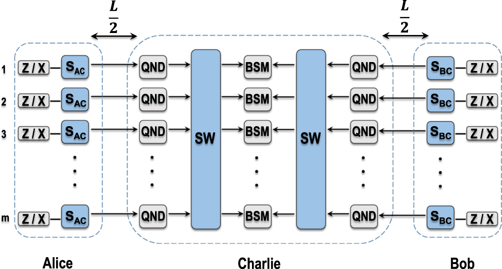
The unit efficiency secret key rate formula can be obtained by noting that in the quantities ${p}_{\mathrm{QND}}$, ${p}_{{\rm{c}}}^{{Z}}$, ${p}_{\mathrm{nc}}^{{Z}}$, ${p}_{{\rm{c}}}^{{X}}$ and ${p}_{\mathrm{nc}}^{{X}}$, given by equations (B18), (B31), (B32), (B47) and (B48) only those terms in which the power of $(1-{\eta }_{\det })$ and $(1-{\eta }_{\det }^{{\prime} })$ is 0 contribute to the sums. This gives restriction on the indices appearing in the power of the terms $(1-{\eta }_{\det })$ and $(1-{\eta }_{\det }^{{\prime} })$. Systematically examining the different cases one by one, we can rule out most of possibilities for the indices. For this, we need to keep in mind that if a sum happens to have a smaller number in the upper limit than that in the lower limit, then the corresponding term gives no contribution to the sum.

Using the recipe given above and the formulas equations (B18), (B31), (B32), (B47) and (B48), we have that

$$\begin{eqnarray}&&{p}_{{\rm{Q}}{\rm{N}}{\rm{D}}}^{[{\eta }_{det}=1,\tau =0]}=\displaystyle \frac{{p}_{1}(2\,{q}_{2}(1-{\eta }_{{\rm{c}}{\rm{h}}})+3{q}_{1}{\eta }_{{\rm{c}}{\rm{h}}})}{48},\end{eqnarray} \tag{ B49 }$$

$$\begin{eqnarray}&&{p}_{{\rm{c}}}^{Z[{\eta }_{det}=1,\tau =0]}={p}_{{\rm{c}}}^{X[{\eta }_{det}=1,\tau =0]}=\displaystyle \frac{{p}_{1}^{2}{q}_{1}^{2}{\eta }_{ch}^{2}}{1024},\end{eqnarray} \tag{ B50 }$$

and

$$\begin{eqnarray}&&{p}_{\mathrm{nc}}^{{Z}[{\eta }_{\det }=1,\tau =0]}={p}_{\mathrm{nc}}^{{X}[{\eta }_{\det }=1,\tau =0]}=0.\end{eqnarray} \tag{ B51 }$$

It is interesting that ${p}_{\mathrm{nc}}^{{Z}}$ turns out to be 0 when we set ${\eta }_{\det }=1$ and $\tau =0\,{\rm{s}}$. In the case considered in the calculations above, Alice and Bob both measured H (horizontal) polarizations in their Z measurement and the two QND measurements succeeded on both side. This means that Charlie's BSM will get input signals in V (vertical) polarizations from both sides. An error can only occur when they apply the bit flip (see step 5 of the protocol), which only happens when Charlie detects a singlet state. But due to the Hong–Ou–Mandel effect the photons will always go to the same arm, therefore in this ideal case Charlie cannot obtain a singlet detection. The same argument holds for the X-basis as well. Plugging equations (B49), (B50) and (B51) into (B5) we obtain the secret key rate formula for the unit detection efficiency case, given by equation (8).