


Abstract
By solving the Bogoliubov–de Gennes equations analytically, we derive the fermionic zero-modes satisfying the Majorana property that exist in vortices of a two-dimensional s-wave Fermi superfluid with spin–orbit coupling and Zeeman spin-splitting. The Majorana zero-mode becomes normalisable and exponentially localised to the vicinity of the vortex core when the superfluid is topologically non-trivial. We calculate the energy splitting due to Majorana hybridisation and identify that the s-wave Majorana vortices obey non-Abelian statistics.
Export citation and abstract BibTeX RIS

Original content from this work may be used under the terms of the Creative Commons Attribution 3.0 licence. Any further distribution of this work must maintain attribution to the author(s) and the title of the work, journal citation and DOI.
1. Introduction
In two dimensions, the quasi-particle excitations of topologically ordered systems are generally non-Abelian anyons [1]. Possible realization of non-Abelian statistics has been studied in connection with the ν = 5/2 fractional quantum Hall (FQH) state [2], and Majorana fermions in the vortex state of chiral  superconductors and superfluids [3–5]. Majorana fermions [6] in the cores of superconductor vortex excitations have been actively considered in the context of p-wave pairing [7–9], but can also occur in an s-wave superconductor coupled by the proximity effect to a topological insulator [10]. Majorana vortices in the topological s-wave superconductor are non-Abelian, and in the same topological class [1] with the Moore–Read Pfaffian FQH state [11, 12],
  superconductors [13, 14], and the gapped non-Abelian spin liquid phase of the Kitaev model [15]. A key benefit of non-Abelian exchange statistics is that the Majorana vortices can be used to realize braiding operations. Non-commutative braiding, which amounts to exchanging two Majorana vortices adiabatically [16], is a key ingredient needed for performing quantum logic operations on a fault-tolerant topological quantum computer [17].
In addition to the importance of a better fundamental understanding of the occurrence of fractional quantum exchange statistics in nature, experimental realization of Majorana fermions in a well-controlled setup carries a lot of significance associated with achieving the non-Abelian properties. Especially important are feasible prospects for the Majorana braiding needed for topological quantum computing and quantum information applications. While much previous attention in the search for Majorana fermions has been given to topological superconductors such as Sr2RuO4 [18], specifically focussing on spinless (chiral) p-wave systems which break time-reversal symmetry [3, 4, 19], the reach of such effectively spin-quenched systems typically lies behind significant experimental barriers.
Fu and Kane [10] proposed an alternative approach where an s-wave (spinful) superconductor is interfaced with a strong 3D topological insulator characterised by time-reversal symmetric topological surface states in the energy gap of the bulk. The proximity effect couples the Cooper pairs of the s-wave superconductor to the topological surface states, physically allowing them to tunnel into the surface states, which gives rise to a topologically non-trivial superconductor that can support Majorana fermions in vortex cores and their non-Abelian statistics. The effective pairing mechanism in the resulting topological superconductor is not dissimilar from p-wave symmetry, but contrary to p-wave superconductors it does not break time-reversal symmetry [10]. Experimental evidence for superconductivity in surface states of a strong topological insulator has been recently reported in thin films of Bi2Te3 grown on a NbSe2 substrate [20]. Later, signatures for Majorana fermions have been experimentally detected in such Bi2Te3/NbSe2 heterostructures [21]. While such a proximity-induced topological s-wave superconductor can support Majorana vortices, the robustness of the Majorana fermions is susceptible to thermal effects. To increase the stability of the Majorana fermions the Fermi energy needs to lie close to the Dirac points, which can be tuned by doping and alloying effects, but whose precise control is still experimentally desired. Moreover, in this limit the superconducting gap becomes small making the proximity effect weaker.
Majorana fermions are also exhibited by generalised interfaces of topological order with superconducting and magnetic order. Sau et al showed that a heterostructure consisting of a regular semiconductor film with spin–orbit coupling sandwiched between an s-wave superconductor and a magnetic insulator realizes non-Abelian Majorana fermions [22]. Proximity of the semiconductor to a magnetic insulator is necessary to explicitly break time-reversal symmetry, making the edge of the semiconductor film an effectively chiral Majorana wire with Majorana fermions at the ends. In a related setup of a one-dimensional semiconductor nano-wire with strong Rashba spin–orbit coupling embedded into a superconducting quantum interference device, but in a real external magnetic field opening a Zeeman gap in the semiconductor without significantly suppressing the superconductor, Majorana fermions were predicted to occur as a function of the external magnetic field [23].
While displaying signatures for Majorana fermions, it remains an open question how to experimentally execute the quantum information and computation aspects using the solid-state approaches where the crystal structure is fixed and vortices are typically pinned which strongly restricts their coherent dynamics. To overcome some of these difficulties a  superfluid has been considered as a platform for topological quantum computation [24]. In current ultra-cold atom experiments [25–27], however, the densities and temperatures are low, and the scattering between fermions takes place typically in the s-wave channel [28]. Here, we theoretically illustrate the Majorana physics in a system of ultra-cold atoms forming a topological s-wave Fermi superfluid with promising experimental control and isolation from environment, where the non-Abelian Majorana braiding and fusion dynamics translates into superfluid vortex dynamics and can therefore arise in a very natural way. Even though the Fermi superfluid is qualitatively a different physical system, the origin of topology in the superfluid arises from analogous ingredients such as superfluid order, spin–orbit coupling, and a Zeeman gap [29]. The (uniform) superfluid becomes topologically non-trivial when
  , where
  is a Zeeman field creating an energy splitting between the spin components,
  is the average chemical potential, and Δ is the superfluid order parameter [30]. The value at equality corresponds to the critical Zeeman field marking a quantum phase transition to the topological regime.
Experimentally, the ultra-cold atomic s-wave Fermi gas is a highly flexible quantum many-body system whose interactions, spin balance, and trapping geometries can be tuned nearly arbitrarily [31, 32]. In the mean-field picture, it is possible to achieve band inversion leading to a topological phase [1, 29] by combining the effects of two-dimensional spin–orbit (SO) coupling [33, 34], and spin imbalance [35, 36]. Recently, tunable 2D SO coupling was demonstrated experimentally [37]. These advances open up a promising perspective for creating a highly-controlled atomic topological superfluid [38, 39] in the laboratory in the near future. In particular, the superfluid allows for a natural setting for studying vortex dynamics, which introduces new avenues for realizing braiding operations. In the superfluid context, possible signatures for the Majorana fermion bound in the vortex core can include its effect on the vortex mass, which can be experimentally probed through e.g. vortex oscillation measurements [40].
Despite the promising recent experimental progress, Majorana zero-modes in vortices of an s-wave Fermi superfluid with SO coupling and a Zeeman field remain relatively poorly understood. Here, we derive analytically the Majorana vortex zero-mode, and use it to calculate the energy splitting due to inter-vortex tunnelling. Due to the qualitatively different microscopic physics, the tunnelling amplitude we derive exhibits a new and different symmetry compared to previous studies on solid-state heterostructures or p-wave systems, which is important for the collective dynamics of more than one Majorana fermion. The tunnelling generally lifts the zero-mode degeneracy [41], and has been studied for the Moore–Read state [42], Kitaev's honeycomb model [43], and p-wave superconductors [44–46]. Hybridisation of Majorana fermions in dense vortex lattices gives rise to a band structure [47–49]. Of particular interest for experimentally controlled quantum simulation are topologically non-trivial bands of Majoranas [50], and the possibility of flattening them [51].
2. Physical system
The Hamiltonian of a two-dimensional Fermi gas with spin–orbit coupling and spin-imbalance reads [52]
where  is the total number of atoms with spin
  , the operator-valued field
  obeys Fermi anti-commutation relations and creates a spin-σ fermion at location
  at time t,
  ,
,  so that
  and
and  . Here
  is a Zeeman field creating an energy splitting between the spin components. The SO coupling is represented by
  with
with  and
and  .
.
We now assume that the two-body interaction is spin-independent,  , and represents contact interactions,
  , where the sign convention is chosen such that
  corresponds to attractive contact interactions.
Superfluidity in spin-balanced Fermi gases results from the formation of Cooper pairs, bound states of two fermions around the Fermi surface with opposite momenta  and
and  . For spin-imbalanced pairing [53], theoretical predictions such as FFLO [54, 55] and Sarma phases [56] together with deformed Fermi surface superfluidity [57] have been presented. In the FFLO phase the Cooper pairs have a non-zero center-of-mass momentum which gives rise to a periodic spatial modulation of the order parameter and also possibly of density. While spin-imbalance can thus influence the pairing and subsequently the dynamics of topological defects by frustrating the Cooper pairing, in experiments the excess non-superfluid particles are typically spatially separated from the completely paired BCS superfluid [36, 58, 59].
In typical current experimental conditions in ultra-cold atoms, the pairs form in the s-wave state with zero angular momentum. The Pauli principle then necessitates that the spin state be a singlet. Since the Cooper pairs have no angular momentum and no net spin, the relative pair wavefunction can be fully characterised by a single complex amplitude  .
.
Ignoring now all the other quantum correlations apart from the pair correlations captured by the order parameter, the mean-field Hamiltonian describing quasi-particle excitations in the superfluid Fermi gas without spin-rotational invariance reads  , where
  is the 4-component Nambu spinor, and
is the Bogoliubov–De Gennes (BdG) matrix representation. In what follows, we are not interested in explicit time dependence and therefore drop the labels.
In the mean-field picture, we replace the many-body problem (1) with the effective single-particle Hamiltonian (2) parametrised by the pair potential (order parameter)  . The pair potential together with the chemical potential is determined by optimising the effective Hamiltonian (2) such that it minimises the total free energy. The result for the pair potential is

and for the atomic densities

where ν labels the discrete energy eigenvalues of the BdG matrix, and ![${f}_{\nu }=1/\left[{{\rm{e}}}^{{E}_{\nu }/({k}_{{\rm{B}}}T)}+1\right]$](https://content.cld.iop.org/journals/1367-2630/21/11/113033/revision2/njpab5336ieqn28.gif) is the Fermi distribution for occupations and T is the temperature. We set T = 0. We have expressed the order parameter in terms of the amplitudes u and v, defined by the Bogoliubov–Valatin transformations
is the Fermi distribution for occupations and T is the temperature. We set T = 0. We have expressed the order parameter in terms of the amplitudes u and v, defined by the Bogoliubov–Valatin transformations ![${\hat{\psi }}_{\sigma }({\bf{r}})={\sum }_{\nu }\left[{u}_{\nu ,\sigma }({\bf{r}}){\hat{\gamma }}_{\nu }+{v}_{\nu ,\sigma }^{* }({\bf{r}}){\hat{\gamma }}_{\nu }^{\dagger }\right],{\hat{\gamma }}_{\nu }^{\dagger }=\int {\rm{d}}{\bf{r}}{\sum }_{\sigma }\left[{u}_{\nu ,\sigma }({\bf{r}}){\hat{\psi }}_{\sigma }^{\dagger }({\bf{r}})+{v}_{\nu ,\sigma }({\bf{r}}){\hat{\psi }}_{\sigma }({\bf{r}})\right]$](https://content.cld.iop.org/journals/1367-2630/21/11/113033/revision2/njpab5336ieqn29.gif) , which diagonalise the effective single-particle mean-field Hamiltonian.
, which diagonalise the effective single-particle mean-field Hamiltonian.
3. Majorana zero-mode in an s-wave Fermi superfluid
3.1. Symmetries of the Hamiltonian
To obtain the static properties of Majorana fermions at the vortex cores in a topological s-wave Fermi superfluid, we need to solve the fundamental eigenvalue equation

for the zero-mode  with
with  . When considering equations of the form (5), it is instructive to first understand the symmetries of the underlying Hamiltonian.
The BdG Hamiltonian  possesses a particle-hole symmetry (PHS) defined by
  with
with  , where K is the complex conjugation operator (in momentum space, K additionally flips the sign of the momentum),
  (
( ) is the Pauli matrix in particle-hole (spin) space, and
  . As a result of the particle-hole symmetry, if
  is a solution of equation (5) with energy Eν, then
  is a solution with energy
  .
.
Additionally, if and only if  and
and  , the BdG Hamiltonian possesses a time-reversal symmetry defined by
 ![$\left[T,H({\bf{r}},t)\right]=0$](https://content.cld.iop.org/journals/1367-2630/21/11/113033/revision2/njpab5336ieqn43.gif) , where
, where  (
( , for half-integer spin), and θ is arbitrary. We have defined
  to be the identity matrix in the particle-hole space, while
  is the Pauli matrix in spin space.
A straightforward calculation shows that non-degenerate zero-modes (that is, the modes  with
with  ), must always satisfy the important symmetry

which is the so-called Majorana property making the zero-mode special. The Majorana property ensures that the quasi-particle operators

satisfy  they represent Majorana fermions.
Let us temporarily assume that time-reversal symmetry is respected, i.e.  and
and  . If
. If  is a solution of equation (5) with energy Eν, then
  is a solution with the same energy Eν. This is the pair of the zero-energy Majorana mode. With time-reversal symmetry, the Majorana probability densities are identically overlapping in space:
  . We need to break the time-reversal symmetry to separate them spatially, for example, by having a vortex in the order parameter. We note that the focus here is on an infinite system where we ignore the boundary physics. Strictly speaking, in the case considered here, there can only be one or zero Majorana zero-modes depending on the topological properties of the superfluid. In experiments the Fermi superfluid is always trapped, where in the topological regime there is a localised state at the edge and at the vortex core which can be identified as Majorana fermions in the thermodynamic limit. This case has been studied self-consistently numerically for harmonic trapping in [60].
A broken time-reversal symmetry T, a broken spin-rotational symmetry (due to spin–orbit coupling), and an unbroken PHS  result in the BdG Hamiltonian
  belonging to the symmetry class D in the Altland-Zirnbauer classification [61]. According to [62], point defects (such as the vortices in the order parameter considered here) with a Hamiltonian that belongs to the class D are associated with a
  -valued topological invariant. This means that in the topologically non-trivial regime the number of exact Majorana zero-modes is given by
  , where W is the sum over all vortex winding numbers, with the rest hybridising in pairs forming a band structure. Generally, when multiple vortices are brought close together, the Majorana zero-modes hybridize into a band structure, leading to complex fermion states at positive and negative energy [47–49]. We calculate the energy splitting in equation (18). For periodic vortex lattices, such as the square and the triangular lattice, the resulting low-energy theory is typically gapped and topologically non-trivial [48].
3.2. Eigenvalue equation for the zero-mode
We now include a vortex in the order parameter

where r and φ are polar coordinates centred on the vortex. Energy considerations require that  at the vortex core. The integer ℓdenotes the vorticity, and
  is a real function of r that vanishes at r = 0. In what follows, we will solve equation (5) analytically for the zero-mode
  that exists in the core of the vortex (8).
For convenience, let us first apply the unitary transformation  , which transforms the basis as
  , and shuffles the zeros in the rows and columns of the Hamiltonian
  (equation (2)) to give

where  and
and

Setting  decouples the spins, and the Hamiltonian reduces to a 2 × 2 BdG matrix corresponding to the Fu-Kane model at neutrality, whose Majorana modes have been considered [63]. This is the low-energy regime near
  , which is the topological transition point in typical p-wave systems. The Majorana zero-modes have also been considered for the Fu–Kane model at
  [45].
[45].
However, here we consider the full 4 × 4 structure of equation (5):


When looking for zero-modes, system (11) can be simplified by using the symmetry property (6), that is, we seek simultaneous eigenstates of the PHS. There are two possibilities for θ, namely  , which both satisfy the Majorana relation. This means that with the final solution we must allow for both possibilities. In both cases, we obtain


a coupled 2 × 2 system, which must be solved for  and
and  .
.
In polar coordinates, the spin–orbit coupling terms read ![${\hat{K}}_{\uparrow \downarrow }({\bf{r}})=\lambda {{\rm{e}}}^{-{\rm{i}}\varphi }\left[{\partial }_{r}-({\rm{i}}/r){\partial }_{\varphi }\right]$](https://content.cld.iop.org/journals/1367-2630/21/11/113033/revision2/njpab5336ieqn73.gif) . Observing the azimuthal symmetry, let us try a separable ansatz with angular momentum eigenstates
. Observing the azimuthal symmetry, let us try a separable ansatz with angular momentum eigenstates

with the assumption that  has no r-dependence. Physically, this approximation treats the vortices as points with only a phase profile. Substitution into system (12) shows that we can eliminate the angular dependence by taking
  and
and  , where
  ,
,  with
with  for
for  and
and  for
for  , and
, and  if
if  respectively. This implies
  and
and  . The only requirement here is that
  . Explicitly, the coupled system (12) then reads


The prime denotes differentiation with respect to r. Below, we solve analytically the coupled system (14) for  and
and  .
.
3.3. Series solution for 

The vortex core (r = 0) is an irregular singular point of equation (14) where numerical methods are inherently unstable. An obvious solution is to start the numerical integration at a point  thus avoiding the singularity, but in this case we need to know accurately the initial condition at the rather arbitrary point r0. It is therefore highly desirable to have analytic solutions, at least around the vortex core. In what follows we solve system (14) using the Wasow method [64], a generalisation of the Fröbenius series method for coupled systems of differential equations with irregular singular points.
The details for solving system (14) are shown in appendix. For definitess, we set  . The result is a series solution for
  around the origin that can be evaluated analytically to arbitrary order, and reads
While  can be finite, the boundary condition
  is forced to keep
  finite at the origin, which results from the series solution for
  starting with the power
  whereas that for
  starts with r0. That one spin component is zero and the other finite at the vortex core has been observed in all numerical studies of the Majorana zero-mode in s-wave Fermi gases [60, 65]. In principle system (14) needs four initial conditions, but requiring that
  be finite at the origin consumes two of them leaving only the two initial conditions
  and
and  in the solution (15).
3.4. Existence of the Majorana zero-mode
The existence of the analytical series solutions (15) alone does not guarantee the existence of a topologically protected Majorana zero-mode. The condition for the physical existence of the zero-mode is that it remain normalisable as  .
.
In the limit  , the kinetic energy and terms in
  can be dropped in system (14) to obtain


Physically, we are interested in only the solutions for system (16) that are normalisable. For example, if  and
and  , the only normalisable asymptotic solution is

where C is a constant. Even then, the solution (17) is normalisable only when  . The value at equality corresponds to the critical Zeeman field marking the phase transition to the topological regime with a uniform order parameter,
  [30], which here is associated with the boundedness of the Majorana zero-mode at infinity. However, it is not straightforward to find initial conditions
  and
and  such that the zero-mode has the desired large-r asymptotics.
In principle,  and Δ must be obtained self-consistently in conjunction with solving the BdG eigenvalue equation. Considering a uniform vortex-free system, we can solve equations (3), (4), and (11) self-consistently to find that the superfluid is topologically non-trivial with the parameters
  . Here all units are measured with respect to
  . We have used the pair binding energy of
  in the renormalisation of the gap equation, which otherwise diverges logarithmically. The pair binding energy determines the state of the Cooper pairs across the BCS-BEC crossover [30]. From equation (17), therefore, we know that with these parameters there is an exponentially decaying asymptotic solution, and we have performed a direct search for
  and
and  that match with this asymptotic behaviour.
We retain terms upto  , and use the analytical solution (15) to evaluate accurate initial conditions for a numerical integration of system (14). The truncated analytical series solution agrees with the numerical integration for
  (figure 1). The analytic series expansion can be developed to arbitrary precision. As expected, the numerical solution becomes unstable as the vortex core is approached, but more importantly it can be used to study the boundedness of the mode as
  . We find a bounded zero-mode in vortices with unit positive circulation with the specific parameter values above for
  and
and  . The full solution including azimuthal dependence is then given by equation (13).
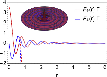
Figure 1. Majorana zero-mode housed by a vortex with unit circulation in an s-wave Fermi gas. The vortex core corresponds to r = 0. The solid lines correspond to numerical integration of system (14), and the dashed lines correspond to the series solution (15) upto  . Inset: revolution plot around the vortex core. Here
  . The initial condition for the numerical evaluation at r = r0 is provided by the analytical solution (15). The zero-mode solution becomes bounded at
  when the superfluid is topologically non-trivial. The parameters are found self-consistently for the uniform vortex-free state, and read
  , and Eb = 0.05. Within numerical accuracy the Majorana zero-mode is normalisable for
  and
and  . We have set
  .
.
Download figure:
Standard image High-resolution image4. Many-body Majorana properties in an s-wave Fermi superfluid
4.1. Majorana energy splitting
We now use the Majorana zero-mode to calculate the energy splitting in an s-wave Fermi gas that results from hybridisation between the Majorana modes of two vortices located at points  and
and  . Then,
  near vortex i (
 ), where
  is the single-vortex pair function (8) for vortex i. Introduction of a single-vortex background phase
  with
with  the azimuthal angle measured with respect to vortex i, amounts to the Majorana mode changing by
  , leaving invariant system (12).
In the tight-binding approximation, the Hamiltonian HΔ describing hopping between the two vortices, whose generalisation to lattices of Majorana vortices requires incorporating a  symmetry (section 4.2), is given by
  , where
  is the Majorana mode (7) at vortex i, and
  is the overlap integral that gives the energy splitting. Here
  is the Majorana zero-mode centered at vortex i.
For convenience, we define  such that
  coincides with equation (10) when the order parameter is given by just a single vortex at position
  . It follows that near vortex 1
  , and the dominant contribution to the overlap integral comes from the vicinity of vortex 2. Taking
  , using equation (13), and introducing the definitions
 ![$G({\bf{r}})\equiv -{\rm{\Delta }}\exp \left[-\tfrac{{\rm{\Delta }}}{\lambda }\left(| {\bf{r}}-{{\bf{r}}}_{2}| +| {\bf{r}}-{{\bf{r}}}_{1}| \right)\right],{{\rm{\Theta }}}_{\sigma {\sigma }^{{\prime} }}({\bf{r}})\equiv {F}_{\sigma }(| {\bf{r}}-{{\bf{r}}}_{2}| ){F}_{{\sigma }^{{\prime} }}(| {\bf{r}}-{{\bf{r}}}_{1}| )$](https://content.cld.iop.org/journals/1367-2630/21/11/113033/revision2/njpab5336ieqn148.gif) , by definition of the zero-mode at vortex 1 we obtain
, by definition of the zero-mode at vortex 1 we obtain

Equation (18) has both oscillatory behaviour and exponential decay in system size (figure 2). The latter is captured by  and the former is captured by
  , which has strong and non-trivial oscillatory dependence on the system parameters as indicated explicitly in system (15) for Fσ.

Figure 2. Majorana tunnelling amplitude ![${\tilde{t}}_{12}={t}_{12}/\left[4\cos \left(\tfrac{{\theta }_{1}-{\theta }_{2}}{2}\right)\right]$](https://content.cld.iop.org/journals/1367-2630/21/11/113033/revision2/njpab5336ieqn151.gif) as a function of vortex–vortex separation
as a function of vortex–vortex separation  (equation (18)). The parameters are the same as in figure 1.
Download figure:
Standard image High-resolution image
4.2. Non-Abelian exchange statistics
Compared to systems with p-wave pairing [66], or the Fu–Kane model [63], in the s-wave Fermi superfluid considered here under Majorana exchange t12 is symmetric with respect to  , but still anti-symmetric overall due to the spin degree of freedom: swopping the vortices amounts to
  . Anti-symmetry of t12 reflects the non-Abelian statistics, and for Majorana vortices in p-wave systems or the Fu–Kane model, where
  , it arises from anti-symmetry with respect to
  .
.
It was pointed out by Fujimoto [1] that the existence of the Majorana zero-mode with SO coupling does not automatically guarantee their non-Abelian statistics. Here, Majorana interchange  gives
gives  , and the U(1) gauge transformation
  of the Majorana fermion has the important property that when
  changes from
  , the Majorana changes sign,
  . Braiding of vortices i and j changes the superfluid phase at one vortex by 2π while leaving the phase at the other vortex invariant, amounting to
  , and it was shown by Ivanov [13] that this property together with quantisation of ℓi gives rise to non-Abelian statistics.
In other words, we can perform a local  gauge transformation
  because the Majorana commutation algebra
  remains invariant. To account for the
  ambiguity when generalising to multiple Majorana vortices we introduce the
  gauge factors
  to the tight-binding Hamiltonian HΔ

where  and given in equation (18). We note that it is Hermitian,
  . Due to the exponential decay of the Majorana zero-mode and the hopping amplitude tij (figure 2), we focus on nearest-neighbour hopping
  only. Since the Majorana fermion corresponds to a zero-energy solution of BdG equations (11), the on-site energy in the tight-binding model is zero leaving only hopping terms. Hamiltonian (19) has been considered in the literature for vortex lattices in the Kitaev spin model on the honeycomb lattice with non-Abelian vortex excitations [14]. Lahtinen [67] extended [43], and mapped the Kitaev spin model to an effective lattice model of Majorana fermions for the vortex excitations described by Hamiltonian (19) by mapping the spin-
 particles to Majorana fermions.
The existence of the Majorana zero-mode (15) has important consequences for the collective dynamics of networks of Majorana vortices. In a vortex lattice, owing to the factors sij in equation (19), a closed loop can enclose a plaquette of the  gauge flux, which is defined by the product of the factors sij along the trajectory. Using the same Hamiltonian HΔ (but different t12), Liu and Franz [48] showed that in the context of Majorana zero-modes in a vortex lattice in a two-dimensional p-wave superconductor and the Fu–Kane model characterising an s-wave superconductor coupled to a Dirac material through the proximity effect, the
  gauge flux through a general polygon formed by n vortices is given by

The same result can therefore be expected to hold also in the s-wave Fermi superfluid despite the different symmetry with respect to the U(1) gauge factors  . Originally, Grosfeld and Stern [2] derived rule (20) for Majorana zero-modes in the context of the Moore–Read
  fractional quantum Hall state [11]. The effective theory for the Moore–Read Pfaffian
  fractional quantum Hall state is analogous to a spinless
  -wave superconductor of composite fermions [2]. It follows directly from equation (20) that there is a non-zero
  gauge flux of
  and π through an elementary triangular and square plaquette, respectively, of the Majorana lattice. A finite gauge flux that alternates between neighbouring plaquettes is typical of Chern systems [68] with the occupied bands in the gapped phases of Hamiltonian (19) being characterised by a non-zero Chern number.
It should be noted that for strict thermodynamic stability of the vortex lattice we need a gauge field  , which in the superconductor context is a magnetic field [48], and in the superfluid context represents rotation [69–71]. The phase difference
  in equation (18) is then replaced by a gauge-invariant version
  , where the integral is along the line segment joining the two vortices [63]. While these terms must be included in any calculation that aims to accurately study the band structure of many-Majorana physics in a thermodynamically stable vortex lattice, the conclusions drawn here are not sensitive to the thermodynamic stability.
5. Discussion and conclusions
We have derived analytically the Majorana zero-mode in a topological Fermi superfluid with s-wave pairing, two-dimensional spin–orbit coupling, and a Zeeman field. The solution can be expected to be of importance for Majorana zero-modes in vortices of solid-state heterostructure systems as well given the mathematically similar Hamiltonians. We find an exponentially localised Majorana zero-mode at the vortex core only in the topologically non-trivial regime of the superfluid. We find that in the s-wave Fermi superfluid the Majorana fermions obey non-Abelian exchange statistics, but exhibit a new symmetry with respect to the underlying U(1) gauge factors, and thus the energy splitting due to Majorana hybridisation is determined by both spin sectors.
Using an s-wave Fermi superfluid as a physical platform for studying Majorana fermions and ultimately realizing hardware for a topological quantum computer inherits many of the features discussed in the context of a p-wave Fermi superfluid [24]. In Fermi superfluids, vortex dynamics including pinning and braiding can be achieved using optical tweezers as long as the tweezer potential is smaller than  [24]. Measurement of vortex locations and dynamics has been experimentally demonstrated in an s-wave Fermi superfluid [72]; phase-contrast imaging can enable non-destructive measurements as well [24]. However, in contrast to the solid-state systems, there is no Coulomb interaction in the neutral superfluid. Instead, we can expect that long-range interactions are mediated in this neutral system via dipole–dipole coupling, which for example occurs in experiments on topological Fermi superfluids using ultra-cold Dysprosium atoms [73].
Knowing the Majorana zero-mode analytically paves the way for studies of quantum many-body correlations and simulation of topological quantum matter in lattices of Majorana vortices in a new experimentally well-controlled setup. One important outlook is the time and space dependent evaluation of the self-consistent Bogoliubov–de Gennes formalism to study vortex dynamics, however, the computational complexity of such a problem is formidable. It might be possible to find important limits where the formalism can be accurately simplified by focussing on a projected spin-quenched system instead [30]. One important prospect is the realization of a fractional Chern insulator to probe quantum Hall physics captured by equation (20), however, it is not entirely clear how to achieve a fractional population of the Majorana bands. Another promising prospect is the realization of Sachdev–Ye–Kitaev (SYK) models [74] with Hamiltonian  , where
  and randomly distributed. The Hamiltonian
  exhibits interesting level statistics [74], and could be realised in the Fermi superfluid by uncertainty in the positions of the vortices giving rise to random fluctuations of tij and gijkl. In summary, the Majorana lattice supported by the topological Fermi superfluid provides a rich platform for simulating topological quantum matter.
Acknowledgments
I would like to thank Andreas Läuchli for fruitful discussions. This work was supported by the Austrian Academy of Sciences (P7050-029-011).
Appendix.: Solution for the Majorana zero-mode
A.1. Formulation as a first-order system
Introducing the first derivatives  and
and  as auxiliary variables, we can trivially regroup system (14) for
  and
and  in terms of
  . This gives the equivalent matrix equation

where
where  . This is a set of linear equations because
  does not depend on the components of
  , but the coefficient matrix
  is non-constant depending on r.
The point r = 0 is an irregular singular point of equation (A1) because the coefficient matrix  has a pole of order 2 at the origin.
Generally, if  , then equation (A1) can be easily solved in terms of the matrix exponential

where  is a 4-component constant vector. However, the commutation property does not hold here. There is no general closed-form solution for differential equations of the form of equation (A1) where
  does not satisfy the commutation property. The Magnus series provides systematically an exact solution in terms of an infinite series of nested commutators:

where


but this approach suffers from the irregular singular point at the origin as well.
Near r = 0, we can always write

where  are constant 4 × 4 matrices holomorphic at r = 0 for which the series converges component-wise in a neighbourhood of the origin. Here g = 2, and
  for only
  .
.
A.2. Solution for the eigenvalue equation (14)
Generalising the vector  into the matrix X, and transforming
  changes equation (A6) into

where  and
and

with the only non-zero matrices being
The matrix  is holomorphic at
  meaning that there exists a convergent expansion of the form (A8) for sufficiently large x0 such that
  . If the integer
  , the singular point is irregular, and if
  , the singular point is regular. For us q = 0. Our goal is to reduce equation (A7) (where q = 0) through formal transformations into a system with
  , which corresponds to a regular singular point at the origin
  , and can be solved in terms of more standard Fröbenius series ansatz methods.
To form our starting point, we transform  into the Jordan canonical form (JCF) (we define the JCF as having the 1's on the superdiagonal). The matrix
  is brought to the JCF by the non-singular constant similarity transformation
where for definiteness we have fixed  .
.  is now in the canonical Jordan block diagonal form

where Hj ( ) are shifting matrices where H1 is of dimension two and
  are of dimension 1. The same transformation is applied to all the matrices, defining the new starting point
  such that

where q = 0, and
A.2.1. Prepare for a shearing transformation that simplifies the problem
The transformation  , where the matrix
  is holomorphic and has a non-vanishing determinant at
  changes equation (A12) into

with  and
and

We seek series solutions  , where we recall
  . We set


Using equation (A16), substitution of the series ansätze into equation (A15) and comparison of like coefficients results in the recursion relation


where the last term in equation (A17b) is absent for  , that is, for ν < 1. The recursion relation is of the form

where  depends only on the
  with j < ν. If all the eigenvalues of
  are distinct, then
  will be diagonal and the problem is uncoupled and easily solved. If at least two eigenvalues are distinct, we can take all
  (ν > 0) zero or block-diagonal. However, this is not possible here because
  has only one distinct eigenvalue, zero.
Instead, we partition each equation (A18) into blocks of the same order as the Jordan blocks Hj for  , and call these blocks
  with
with  . For us s = 3. Then each relation (A18) corresponds to s2 = 9 relations

It can be proven that the equation  possesses solutions other than X = 0 if and only if A and B have at least one common eigenvalue. Since this result guarantees the existence of non-trivial solutions to the corresponding homogeneous equations of equation (A19), each equation of equation (A19) can be soluble only if the matrices
  satisfy some restrictive condition, explained below. Consider the auxiliary equation

where H and K are shifting matrices of orders h and k respectively, and M is a h × k matrix whose first h − 1 rows are given constant vectors while the entries α1, α2, ..., αk of the last row are variables. It can be proven that the numbers α1, α2, ..., αk can be determined uniquely in such a way that equation (A20) is solvable for the h × k matrix X. We now apply this result to equation (A19). Without loss of generality we take all rows but the last of  to be zero. Then, the series

is determined by solving the recursion relations (A19) successively for ν = 1, 2, .... While it will in general be divergent, it can be proven that it is the asymptotic expansion of some holomorphic matrix function  for sufficiently large x0 such that
  .
.
The point of the transformation  is to obtain a differential equation (A14) such that the matrices
  , by construction, satisfy the following three properties: (i)
  (ii)
(ii)  (the Hj are shifting matrices); and, most importantly, (iii) that the only non-zero entries in
  for ν > 0 occur in the rows corresponding to the last rows of the Jordan blocks Hk (k = 1, 2, ..., s) in the representation of
  . The transformation
  induces zeros into the matrices preparing them for a shearing transformation. The result is an asymptotic series solution valid at
  such that
  , where

We work until  . The final series solutions will then be exact upto
  for
for  and
and  for
for  . For spin-
 the derivative (component 2) will agree with a direct derivative of component 1 upto
  and for spin-
 the derivative (component 4) will agree with a direct derivative of component 3 upto
  .
.
A.2.2. Simplify the problem by a shearing transformation
Having obtained the matrix  , equation (A14) is ready for the shearing transformation

with a temporarily unknown positive parameter ξ, which takes equation (A14) into

where the matrix  . The matrix elements cjk (
 ) of
) of  read
read

Here δjk is the Kronecker delta, and bjk are the matrix elements of  . The parameter ξ must be chosen appropriately to induce, where possible, non-zero elements below the main diagonal into the leading order matrix
  . Above the main diagonal it is equal to
  .
.
The parameter ξ must be chosen judiciously as follows. Any  is of the form

where  and each positive integer
  except for the special elements with a 1 from a shifting matrix in the Jordan decomposition for
  for which αjk = 0. Since we could not diagonalise
  and instead obtained a Jordan matrix, at least one such special element is present. Before the shearing transformation (
 ) the special elements have the lowest αjk, and the purpose of the transformation is to add non-zero elements on or below the diagonal to
  by a suitable choice of ξ. After the shearing transformation the expansions of non-zero off-diagonal elements cjk (δjk = 0) begin with the power
  . The special elements on the superdiagonal begin with the power
  . There exists a smallest rational
  with
with  coprime, for which the special elements have the same leading power as an element below the main diagonal,
  for some j, k < j. We take ξ = ξ0 in the shearing transformation; the result of the above process is
  with
with  coprime. Fractional powers thus unavoidably appear in the shearing transformation (A23).
In descending powers of  , the matrix
  will begin with the power
  . The matrix
  as
as  has at least one non-zero entry on or below the main diagonal and above the main diagonal it is equal to
  :
:
We remove the fractional powers by multiplying both sides by  and introducing the new independent variable x1 such that

to obtain from equation (A24) the differential equation

where

The branch of the multi-valued function  can be chosen freely.
While new elements have appeared on and below the main diagonal in  , the upper triangular part above the main diagonal, in particular the superdiagonal, of
  is equal to that of
  by construction. This completes the purpose of the shearing transformation.
If  , the problem would be solved because then either the singular point would be regular (
 ), or there would not be any singular point. If
  and
and  has at least two distinct eigenvalues, then the problem reduces to a set of similar problems of lower order. However, the eigenvalues of
  are all equal to zero, and
  is nilpotent. It can be proven [64] that if the process outlined above is repeatedly carried out, eventually we obtain a nilpotent
  that is itself a shifting matrix i.e. s = 1.
A.2.3. Obtain an equation with a regular singular point
The entire process must be reapplied, starting from the JCF for  . Another shearing transformation with the parameter 1/2 is required. Repeating the process once more, the third shearing transformation comes with an integer-valued shearing parameter of 1, which means that via such a chain of transformations we have reduced the coupled system (A12)

to the system

where
and  . We have reached our goal that we set below equation (A7): equation (A32) has only a regular singular point at infinity (or the vortex core in terms of r). This equation can be solved using more standard methods.
Through a sequence of standard double transformations that raise the eigenvalues of a Jordan block of  by an integer followed by a non-singular constant similarity transformation of
  to JCF, we obtain

such that no eigenvalues of the leading matrix  differ by a positive integer. In fact, it consists of two identical Jordan blocks:
  .
.
Let us now transform back to radial coordinates with  (here
(here  ) to obtain from equation (A34) the equation

where  and
and  is holomorphic.
Since  is holomorphic at
  and since no two eigenvalues of
  differ by a positive integer, equation (A35) has a fundamental matrix solution of the form

where  is holomorphic. Its power series representation
  can be calculated by rational operations from the coefficients
  in the series
  .
.
The matrix  in the transformation
  , which results in the equation

is calculated using the recursion relation (A17) with  and
and  (also changing the sign of the last term in equation (A38b)), viz.


where


Given that the matrix  in the convergent expansion
  has no eigenvalues that differ from each other by positive integers, there exists a formal convergent series
  with
with  such that the formal transformation
  reduces the differential equation (A35) to the form of equation (A37) such that
  for all ν > 0. Therefore, the recursion relations (A38) can be solved for
  such that
  for ν > 0. The solution for
  is then given by equation (A36).
Since ![$\left[\tfrac{{{ \mathcal B }}_{0}^{(7)}}{{r}_{1}},\tfrac{{{ \mathcal B }}_{0}^{(7)}}{{r}_{2}}\right]=0$](https://content.cld.iop.org/journals/1367-2630/21/11/113033/revision2/njpab5336ieqn331.gif) , the general solution to the equation
, the general solution to the equation

is given by the matrix exponential (A3)

Here a set of four linearly independent vectors forms the fundamental matrix solution  , and ϒ(r0) is the fundamental matrix solution at r2 = r0. We can set the auxiliary parameter r0 = 1 and choose ϒ(r0) in such a way as to choose the boundary conditions for Fσ(r) at r = 0. The general (vector) solution is then given by linear combinations of the columns.
The logarithms of the fundamental solution matrix end up in columns 2 and 4 making them either divergent or zero at the origin r = 0. The columns 1 and 3, in contrast, can be chosen to remain well-behaved and finite at the vortex core r = 0. We do not include the columns 2 and 4 in what follows, that is, we take a linear combination only of columns 1 and 3.
Performing all the transformations carried out in an inverse order, we can compute the matrix solution X for the original problem (14) from knowing ϒ(r2). A judicious choice for ϒ(1) (with r0 = 1) then gives the explicit solution shown in equation (15) in the main text.