


Abstract
Neuromorphic photonics is a new paradigm for ultra-fast neuro-inspired optical computing that can revolutionize information processing and artificial intelligence systems. To implement practical photonic neural networks is crucial to identify low-cost energy-efficient laser systems that can mimic neuronal activity. Here we study experimentally the spiking dynamics of a semiconductor laser with optical feedback under periodic modulation of the pump current, and compare with the dynamics of a neuron that is simulated with the stochastic FitzHugh–Nagumo model, with an applied periodic signal whose waveform is the same as that used to modulate the laser current. Sinusoidal and pulse-down waveforms are tested. We find that the laser response and the neuronal response to the periodic forcing, quantified in terms of the variation of the spike rate with the amplitude and with the frequency of the forcing signal, is qualitatively similar. We also compare the laser and neuron dynamics using symbolic time series analysis. The characterization of the statistical properties of the relative timing of the spikes in terms of ordinal patterns unveils similarities, and also some differences. Our results indicate that semiconductor lasers with optical feedback can be used as low-cost, energy-efficient photonic neurons, the building blocks of all-optical signal processing systems; however, the length of the external cavity prevents optical feedback on the chip.
Export citation and abstract BibTeX RIS

Original content from this work may be used under the terms of the Creative Commons Attribution 3.0 licence. Any further distribution of this work must maintain attribution to the author(s) and the title of the work, journal citation and DOI.
1. Introduction
The nonlinear dynamics of semiconductor lasers with optical feedback has been intensively investigated [1, 2], not only because of its interest as an experimental test bed to study nonlinear phenomena, but also, because it has found many practical applications [3], including random number generation [4–7], photonic microwave generation [8–10], chaotic lidar [11], compressive sensing [12] to name just a few. Recent experimental and theoretical studies have demonstrated that the high-dimensional feedback-induced dynamics can be exploited for neuromorphic computing, using the reservoir computing paradigm [13–16]. On the other hand, intensive research has focused on the implementation of photonic neurons, able to perform pattern recognition, logic operations and calculations [17–25]. A promising optical system for neuromorphic applications is an optically injected semiconductor laser that displays excitable optical pulses [26–29]; however it has the disadvantages that it needs the use of an optical isolator (or circulator) to avoid back reflections and is sensitive to small changes in the wavelength of the injected light (that can be produced, for example, by temperature or pump current fluctuations).
It is well-known that optical feedback can induce excitable dynamics in semiconductor lasers [30–34]. In the regime known as low frequency fluctuations (LFFs) the laser intensity displays abrupt and irregular power dropouts (see figure 1) that resemble the spikes fired by a neuron (see figure 2). The laser spiking output can be used for implementing a photon neuron; however, it is important to first investigate to what extent the dynamics of the laser mimics the neuronal dynamics. In particular, it is important to quantify similarities in the spike timing and in the spike rate, as single neurons and neuronal populations use spike sequences to encode information. Spike sequences can contain information based on different coding schemes, for example, the information can be encoded on the average firing rate ('rate code') or in the timing of single spikes ('temporal code') [35–37].

Figure 1. Example of the experimental intensity time series (solid line) and the signal that modulates the laser current (dashed line). In panel (a) no modulation is applied; in panel (b), the modulation amplitude is 2.4% of Idc and the period is 143 ns.
Download figure:
Standard image High-resolution image
Figure 2. Example of the simulated neuronal spikes (u(t), solid line) and the modulating signal (dashed line). In panel (a) no modulation is applied; in panel (b), the modulation amplitude is 0.07 and the period is 3.7, both in arb. units; other parameters are as indicated in the text.
Download figure:
Standard image High-resolution imageA first step in this direction was done in [38], where it was shown that in the LFF regime, spike correlations can be described by a simple minimal model, a modified circle map, that also describes temporal correlations in spike sequences of real neurons [39]. Specifically, in [38] the circle map was found to qualitatively describe the statistics of a sequence of symbols, known as ordinal patterns (OPs) [40], defined from the laser interspike intervals (ISIs). Follow up studies have analyzed how the statistical properties of the laser spikes are affected by a periodic modulation of the laser current [41–43].
However, the similarity between the laser spikes and the neuronal spikes has not yet been investigated. Here we compare the statistical properties of the spikes emitted by the laser with neuronal spikes simulated using a well-known model, the stochastic FitzHugh–Nagumo (FHN) model [44–47]. The FHN model has two rate equations, one for a fast variable that represents the voltage of the neuron's membrane, and a slow variable that represents the refractory properties of the neuron. We analyze experimentally how the laser spike rate varies with the amplitude and with the frequency of the signal that directly modulates the laser current, considering sinusoidal and pulsed waveforms, and show that, in both cases, a qualitatively similar behavior is predicted by the FHN model. In both forced systems chaotic behavior can also be expected and a detailed comparison of the attractors will be interesting; however, here we focus only in the similarities in the spike rate and in the timing of the spikes because the spike rate and the spike timing can be used for information encoding.
We also compare the laser spikes with the neuronal spikes using OP analysis [38, 40]. This is a popular technique to investigate complex signals, which has been extensively used to characterize the dynamical regimes of semiconductor lasers with optical feedback [41, 48–57]. A main advantage of this methodology is that, in its simplest implementation, it has only one parameter that is the size, D of the pattern, which determines the length of the temporal correlations studied: the D! different patterns (or symbols) are obtained from the relative ordering of D consecutive data points, without the need of explicitly defining one or more threshold values for partitioning the phase space. Using ordinal analysis we uncover similarities, but also differences, between optical and neuronal spikes.
This paper is organized as follows. Section 2 describes the experimental setup, section 3 presents the FHN model, section 4 presents the results, and section 5 presents the conclusions.
2. Experimental setup
The experimental setup is as described in [42, 43]. A semiconductor laser (685 nm Thorlabs HL6750MG with solitary threshold  mA), has part of its output fed back to the laser by a mirror. The feedback produced a 7.2% threshold reduction (
 mA). The length of the external cavity is 70 cm, which gives a delay time of 5 ns. The laser temperature and current were stabilized with 0.01 C and 0.01 mA accuracy, respectively. A 90/10 beam-splitter in the external cavity sends light to a photodetector (Det10A/M), an amplifier (Femto HSA-Y-2-40), and a 1 GHz oscilloscope (Agilent DSO9104A). The laser is electrically pumped through a 500 MHz bias-tee that combines a constant dc current, Idc = 26 mA, with a periodic signal from a function generator (Agilent 81150A). Sinusoidal and pulsed waveforms were used. The duration of the pulse was the shortest available: 5 ns with raising and falling times of 2.5 ns each. The modulation frequency was varied from 1 to 80 MHz in 79 steps of 1 MHz each. The spike rate of the laser without modulation is 3.3 MHz.
The peak to peak modulation amplitude was varied from 0.19 to 0.631 mA in 7 steps of 0.063 mA. Therefore, the modulation amplitude, for the dc value of the pump current used during the experiment, 26 mA, represents a variation between 0.8% and 2.4% of the dc level.
A LabVIEW program was used to control the experiment and for each set of parameters, intensity time series with 107 data points were recorded with 2 GS s−1 sampling rate, which allowed to capture the intensity dynamics during 5 ms. Figures 1(a) and (b) (without and with modulation respectively) display a short time interval (2 μs) during which typical abrupt drops of the intensity (referred to as spikes) can be seen. The spikes are irregular in the absence of current modulation, and become regular when the external signal modulates the laser current.
The intensity time series typically contains more than 104 spikes. The ISIs are ΔTi = ti − ti−1, where ti are the spike times, which were detected using the same method as in [42, 43]. First, each time series is normalized to unit variance (the dc value is removed by the amplifier, so the time series has zero mean). Then, a spike is detected whenever the intensity drops below a threshold, equal to −1.5 in units of the standard deviation. To avoid detecting as spikes the fluctuations that occur during the recovery process, the intensity has to grow above the zero mean value, before another spike can be detected.
3. Neuron model
The FHN model [44, 45] is a popular simple model of neuronal activity. The model equations are:


where the two dimensionless variables u and v are a fast voltage-like variable and a slow recovery-like variable, also called activator and inhibitor variables, respectively; s(t) represents an external input signal, and ξ(t) represents Gaussian white noise of intensity D. a and  are parameters that control the spiking activity of the neuron: for
  without any perturbation (D = s = 0) the neuron fires periodic (tonic) spikes, while for
  the neuron is in the excitable regime: if a small perturbation occurs (below a certain threshold) the neuron returns to the stable state after a small oscillation. On the contrary, if the perturbation is above the threshold, then, there is a large excursion in the phase space, which is known as action potential or spike. After the spike the neuron returns to the rest state and a refractory period follows during which another perturbation can not trigger another spike.
The input signal s(t) is periodic, with sinusoidal or pulsed waveform. For a precise comparison the same signal that modulates the laser current is used; however, to trigger spikes the pulsed waveform is inverted, as shown in figure 2 (the signal is also re-scaled in time, in order to vary the frequency). In the FHN model the signal is included in the rate equation of the fast variable because of the biophysical mechanisms of spike generation (sufficiently large inputs change the neuron's membrane potential and generate electrical pulses, known as action potentials or spikes); in contrast, in the laser the signal is applied to the pump current, which modulates the carriers (electron–hole pairs), which are coupled to the intensity dynamics through light–matter interactions.
The FHN model equations were simulated with parameters in the excitable regime, a = 1.05, = 0.02 and D = 10−5. For these parameters the natural spike rate of the neuron (without the external signal) is 0.12 arb. units. The signal amplitude was varied between 0.03 and 0.07, and the signal frequency was varied from 0.02 to 1.2 arb. units. These values were found to give a good agreement with the empirical laser data.
Time series containing 104 spikes were generated from random initial conditions, Examples of the simulated neuronal spikes are displayed in figure 2.
4. Results
We begin by analyzing how the distribution of inter-spike intervals (ISI distribution) depends on the frequency of the external signal. Figure 3 displays in color code the ISI distribution for the empirical laser ISIs (a), (b) and for the simulated neuronal ISIs (c), (d). The signal waveform is sinusoidal in panels (a), (c) and pulsed in panels (b), (d). The ISI values are normalized to the period of the signal, Tmod; therefore, the plateaus seen for ISI/Tmod = 1, 2, 3, ... reveal the characteristic locking structure of periodically forced excitable systems [58, 59] that has been observed experimentally in semiconductor lasers with optical feedback [42, 43, 60]. In the following, locking n:1 means that the laser, or the neuron, emits a spike every n cycles of the modulation.

Figure 3. Interspike interval (ISI) distribution as a function of the frequency of the signal for (a), (b) the laser ISIs with a modulation amplitude of 0.62 mA (2.4% of Idc), and for (c), (d) the simulated neuronal ISIs with amod = 0.07. The modulation waveform is sinusoidal in (a), (c) and pulsed in (b), (d). In order to enhance the plot contrast, the color scale indicates the logarithmic of the number of ISIs (the white color stands for zero counts). The vertical axis displays the ISI normalized to the period of the signal.
Download figure:
Standard image High-resolution imageFor the laser ISIs, with sinusoidal modulation, figure 3(a), locking regions 2:1 and 3:1 are observed, located at ∼30 MHz and ∼50 MHz, respectively. With pulsed modulation, figure 3(b), at lower frequencies locking 1:1 is also seen [for 7 MHz the intensity time series was shown in figure 1(b)]. With both waveforms, at higher frequencies the laser is unable to lock and the ISI distribution is multi-modal. The waveform affects the laser ISI distribution mainly at low frequencies (below ∼30 MHz).
For the neuron ISIs, with sinusoidal modulation, figure 3(c), locking regions 2:1, 3:1 and 4:1 are clearly observed as narrow plateaus. At low frequencies, there is a wider plateau that corresponds to noisy 1:1 locking. In contrast to the laser, even at high frequencies (not shown) the neuron ISIs show locking plateaus, multimodal peaks being observed only during the transitions between n:1 and (n + 1):1 locking. With the pulsed waveform, figure 3(d), the locking is noisier, as revealed by wider plateaus, in comparison with the plateaus produced by the sinusoidal waveform.
The locking plateaus in the four panels of figure 3 reveal that at low frequencies the laser and the neuron ISI distributions agree qualitatively well for both, the sinusoidal and the pulsed waveforms, while at high frequencies the responses of the laser and the neuron are different. A possible reason could be the fact that the signal does not modulate the laser intensity but the laser current. Another possible reason is the fact that the intensity spikes (what we observe in the experiments our 1 GHz oscilloscope) are actually the envelope of a fast pulsing dynamics [2] and fast current modulation affects this underlying pulsing dynamics, but does not produce faster spikes.
Next, we characterize the laser and the neuron responses to the external signal by analyzing how the average spike rate (the inverse of the mean ISI) depends on the signal's amplitude and frequency. The results are presented in figure 4 that displays in color code the spike rate for sinusoidal (figures 4(a), (c)) and pulsed (figures 4(b), (d)) waveforms for the laser ISIs (figures 4(a), (b)) and for the neuron ISIS (figures 4(c), (d)).

Figure 4. The average spike rate (i.e. the inverse of the mean ISI) in color code versus the amplitude and the frequency of the signal, for (a), (b) the laser ISIs and for (c), (d) the neuron ISIs. The signal waveform is sinusoidal in (a), (c) and pulsed in (b), (d).
Download figure:
Standard image High-resolution imageFor the laser, the maximum spike rate, of about 18 GHz, is obtained with the pulsed waveform, figure 4(b), with frequencies of ∼15 GHz, ∼30 GHz, or ∼50 GHz (i.e. in the 1:1, 2:1, or 3:1 locking regions respectively). With the sinusoidal waveform, figure 4(a), locking 1:1 is not seen. At high frequencies the spike rate is similar for both waveforms.
For the neuron, the variation of the spike rate with the signal's amplitude and frequency is qualitatively similar to the laser. In this case, for the lower amplitudes the locking regions are wider for the sinusoidal waveform than for the pulsed one. We speculate that this difference might be due to the fact that the sinusoidal signal affects the neuron's firing threshold all the time, while the pulsed signal only acts during pulses.
In the FHN model theoretical and numerical studies have shown that, without noise, the signal is subthreshold (i.e. it does not induce spikes) if its period is long enough [61, 62]. Our results consistently show that, at low frequencies, the spike rate of the laser and of the neuron is almost unaffected by the signal (blue regions at low frequencies in the four panels of figure 4).
To investigate if there are similarities beyond the average spike rate, we analyze the relative timing of the spikes by applying ordinal analysis [40] to the ISI sequences of the laser and of the neuron. The method consists of transforming each ISI sequence,  , into a sequence of symbols, known as OPs, which are defined by considering the relative length of D consecutive ISIs. For instance, for D = 2 there are two possible OPs: when
  , the pattern is 01, while when
  , the pattern is 10. For D = 3, we have 3! = 6 possible OPs: 012 (ΔT3 > ΔT2 > ΔT1), 021 (ΔT2 > ΔT3 > ΔT1), 102 (ΔT3 > ΔT1 > ΔT2), 120 (ΔT2 > ΔT1 > ΔT3), 201 (ΔT1 > ΔT3 > ΔT2) and 210 (ΔT1 > ΔT2 > ΔT3). As in previous works [38, 55, 56, 62, 63] we use D = 3, which allows identifying temporal relations among four consecutive spikes. As the number of possible patterns increases as D!, a larger D significantly increases the data requirements, because very long sequences of spikes are needed for a robust estimation of the probabilities of the D! OPs.
The results are presented in figures 5 and 6 that display in color code the probability of each OP, for the laser ISIs and for the neuronal ISIs respectively, as a function of the signal's amplitude and frequency. The white color indicates the non statistical significance (NSS) region, where the probabilities are all similar and consistent with the uniform distribution (all the probabilities are the range  , where p = 1/6 and N is the number of OPs [38]). In these plots we see some similarities, but also, some differences. For both waveforms, in wide parameter regions the 'trend' patterns 012 and 210 (three increasingly longer or increasingly shorter intervals, respectively) tend to be less expressed than in a random situation (the blue regions indicate p < 1/6). We also note that the probabilities of the other patterns are similar in pairs: panels (b) and (c), which correspond to patterns 021 and 102, and panels (c) and (d), which correspond to patterns 120 and 201, tend to have similar structure, particularly in the case of the laser ISIs. On the other hand, we see that in the case of the laser ISIs at high frequencies, there is a large red region where pattern 210 is more probable, which is not seen in the neuronal ISIs.

Figure 5. Ordinal pattern probability (in color code) computed from the laser ISIs, as a function of the signal's amplitude and frequency. In the left panels, the waveform is sinusoidal; in the right panels, is pulsed. The labels indicate patterns (a) 012, (b) 021, (c) 102, (d) 120, (e) 201 and (f) 210.
Download figure:
Standard image High-resolution imageTo summarize the information in figures 5–7 displays in color code the most probable pattern, as a function of the signal's amplitude and frequency, for the laser ISIs ((a), (b)), and for the neuron ISIs ((c), (d)), with sinusoidal ((a), (c)) or pulsed ((b), (d)) waveform. Because patterns 021 and 102, and also, patterns 120 and 201, were found to have similar probabilities in the laser ISIs (figure 5) and also, in the neuronal ISIs (figure 6), in these colormaps we merged each pair in a single color. The white color represents the NSS situation, in which the probabilities are consistent with the uniform distribution.
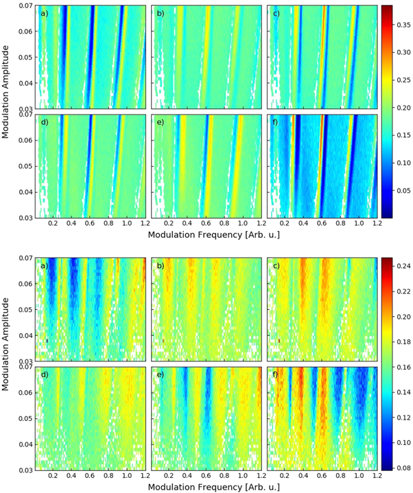
Figure 6. As in figure 5, but for the neuronal ISIs, simulated with the FHN model.
Download figure:
Standard image High-resolution image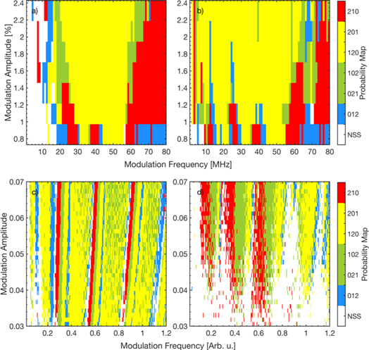
Figure 7. Most probable ordinal pattern (in color code) in the laser ISIs (a), (c) and in the simulated neuronal ISIs (b), (d), as a function of the signal's amplitude and frequency. The modulation waveform is sinusoidal in (a), (c) and pulsed in (b), (d). The white color indicates non-statistically significant (NSS) difference, i.e. all the ordinal patterns have similar probability.
Download figure:
Standard image High-resolution image
For the laser, with sinusoidal or pulsed modulation (figures 7(a), (b)), large yellow regions are seen that have a similar structure as the red regions in figures 4(a), (b). The boundaries of the yellow regions correspond to the transition regions between different locking regimes.
Under sinusoidal modulation, figure 7(a), the low frequency border of the 2:1 locking region is located between 20 and 30 MHz, depending on the modulation amplitude. In this region the sequence of patterns is 012 (blue), 021-102 (green) and 210 (red). For the lowest amplitude, the small red-blue region at 40 MHz corresponds to the transition between locking 2:1 and 3:1. These findings are in good agreement with previous results [38], where it was found that, when increasing the amplitude of sinusoidal current modulation (keeping constant the modulation frequency), pattern 210 (red) is more probable for small amplitude, and patterns 120-201 (yellow) become more probable at higher amplitudes (figure 4(a) in [38]). In addition, the red–blue–yellow transitions seen for the lowest modulation amplitude, when increasing the modulation frequency, agree well with the probabilities presented in [41], figure 6(c). The specific frequency ranges where the different patterns dominate can be expected to be different for different lasers, as they depend on various parameters (e.g. the noise and the dc value of the pump current). A detailed analysis is left for future work.
Under pulsed modulation, figure 7(b), stripes that correspond to the boundaries of the locking regions 1:1, 2:1 and 3:1, located about 14, 25 and 40 MHz, can be seen. These stripes are narrower than in the sinusoidal case but the most probable symbols are the same.
For the FHN neuron, figures 7(c) and (d), wide yellow areas are also seen, but they are more fuzzy than in the case of the laser. We also note that the sinusoidal waveform produces better defined regions, in comparison to the pulsed one. As discussed before, this can be due to the fact that the sinusoidal waveform continuously changes the firing threshold, while the pulsed waveform, changes the threshold only during the pulses. Our findings are consistent with previous work [63], where patterns 120-201 (yellow) or 021-102 (green) were found to be more probable, depending on the modulation period and the noise level.
At low modulation frequencies, we note that the analysis of the spike rate (figure 4) did not reveal an important effect of the external signal, both, for the laser and for the neuron, for the pulsed and for the sinusoidal waveform (the blue regions at low frequencies in the four panels of figure 4 indicate that the spike rate is rather unaffected by the signal); however, in figure 7 ordinal analysis unveils differences in the more probable OP. On the other hand, at high frequencies, in the laser patterns 210 (red) or 012 (blue) are more probable, while in the neuron, patterns 120 and 201 (yellow) and 021 or 102 (green) are more probable. This difference can be due to the fact that at high frequencies the neuron still locks to the signal, while the laser does not.
5. Conclusions
We have studied experimentally the dynamics of a semiconductor laser with optical feedback and current modulation, and compared the intensity spiking dynamics with the dynamics of a FHN neuron, which is modulated with the same input signal that modulates the laser current (sinusoidal or pulsed). We have compared the ISI distributions and found a good qualitative agreement at low modulation frequencies. We have also compared how the laser's spike rate and the neuron's spike rate depend on the amplitude and on the frequency of the signal, and found a qualitative good agreement. Using symbolic ordinal analysis we have also found similarities in terms of the most probable symbols that occur in the locking regions, but we have also uncovered differences at low and high frequencies.
Our results indicate that under appropriated conditions, the laser's spike rate can emulate a neuron's spike rate. Therefore, it could act as a photonic neuron in neuromorphic systems that use spike rate coding for information processing. A drawback of this implementation is that the optical feedback comes from a long external cavity, which prevent the laser integration in a microchip. As future work, it will be interesting to investigate the neuromorphic possibilities of the laser dynamics, when the optical feedback comes from a very short external-cavity. It will also be very interesting to compare the laser and neuron responses to aperiodic signals.
Acknowledgments
This work was supported in part by the Spanish Ministerio de Ciencia, Innovación y Universidades (PGC2018-099443-B-I00). CM also acknowledges partial support from ICREA ACADEMIA, Generalitat de Catalunya.