


Abstract
The function of biological membranes is controlled by the interaction of the fluid lipid bilayer with various proteins, some of which induce or react to curvature. These proteins can preferentially bind or diffuse towards curved regions of the membrane, induce or stabilize membrane curvature and sequester membrane area into protein-rich curved domains. The resulting tight interplay between mechanics and chemistry is thought to control organelle morphogenesis and dynamics, including traffic, membrane mechanotransduction, or membrane area regulation and tension buffering. Despite all these processes are fundamentally dynamical, previous work has largely focused on equilibrium and a self-consistent theoretical treatment of the dynamics of curvature sensing and generation has been lacking. Here, we develop a general theoretical and computational framework based on a nonlinear Onsager's formalism of irreversible thermodynamics for the dynamics of curved proteins and membranes. We develop variants of the model, one of which accounts for membrane curving by asymmetric crowding of bulky off-membrane protein domains. As illustrated by a selection of test cases, the resulting governing equations and numerical simulations provide a foundation to understand the dynamics of curvature sensing, curvature generation, and more generally membrane curvature mechano-chemistry.
Export citation and abstract BibTeX RIS

Original content from this work may be used under the terms of the Creative Commons Attribution 3.0 licence. Any further distribution of this work must maintain attribution to the author(s) and the title of the work, journal citation and DOI.
1. Introduction
Animal life is characterized by a hierarchical compartmentalization into separate functional units delimited by interfaces. At cellular and sub-cellular scales, the fundamental structure supporting compartmentalization is the lipid membrane. To form specialized organelles, lipid membranes must adopt a variety of shapes including spherical vesicles, sheets, tubes, and complex assemblies involving several of these elements [1]. Furthermore, biomembranes need to dynamically reconfigure their shapes and topologies to accomplish vesicular transport [2], cell division [3], or to unfold membrane reservoirs under stress [4]. The plasma membrane is also a mechanical organizer of the cell [5], and supports a variety of mechanotransduction mechanisms [6]. To perform all these functions, lipid membranes rely on a combination of solid-like mechanical properties, e.g. bending and stretching elasticity, in-plane fluidity, and the interaction with a myriad of curved membrane proteins. Molecularly, membrane proteins impinge curvature on the membrane through various mechanisms, which include curved scaffolding domains, wedge-like insertions [7–9], or asymmetrical crowding of bulky disordered domains [10] or anchored polymers [11] as in the glycocalyx [12] interacting at a distance from the bilayer mid-plane. Here, we refer to all these objects as curved proteins. Besides enabling shape remodeling, membrane fluidity allows curved proteins to migrate to regions of favorable curvature during curvature sensing [13], to cluster and reshape the membrane during curvature generation [7], while membrane tension controls the (dis)assembly of protein-rich curved domains [4].
To quantitatively understand these phenomena, various biophysical studies have exposed artificial lipid membranes to purified proteins in controlled conditions [14]. At high concentration, curved proteins can induce severe membrane curvature when incubated with liposomes [15], can stabilize membrane tubes [10, 16], and can dynamically trigger protein-rich tubular protrusions out of tense vesicles [17–19]. At lower concentrations, proteins sense curvature and preferentially adsorb or migrate to favorably curved membranes, as probed in assays involving polydisperse vesicle suspensions [20], vesicles with membrane tethers [18, 21] or supported lipid bilayers on wavy substrates [22]. Since protein-rich curved domains sequester apparent membrane area from the adjacent planar membrane, their formation perform work against membrane tension, and thus can be hindered if tension is large enough. This kind of mechano-chemical coupling, tested in vitro by exposing aspirated vesicles to BAR proteins [19], has physiological implications during the mechano-protection of stressed cells by the release of membrane area through disassembly of caveolae [4], or in the regulation of clathrin-mediated endocytosis by membrane tension [23].
A number of theoretical and computational studies at various scales have been developed to understand the interaction between curved proteins and membranes. At the nanoscale, all-atom molecular dynamics have described curvature generation by single domains [24] and curvature maintenance by multiple proteins [25]. Reaching a micron, coarse-grained molecular dynamics simulations, treating the membrane either molecularly or as a continuum object, have followed the aggregation of multiple proteins to cooperatively form protein-rich curved domains [26–30]. Models treating proteins as discrete objects in a continuum membrane have examined membrane-mediated protein–protein interactions [31, 32], or the spontaneous curvature induced by anchored polymers [33, 34]. A fundamental obstacle to develop mean field theories at larger scales based on models where proteins are discrete object, however, is the non-additive nature of membrane-mediated pairwise interactions [35]. Reaching larger scales, continuum models combining the Helfrich curvature energy [36, 37] with thermodynamic models of mixtures [38, 39] have been quite successful in recapitulating and interpreting quantitative in vitro measurements, see [40, 41] for two recent reviews. These models suggest that, rather than two different mechanisms, curvature sensing and generation are two manifestations of the same mechano-chemical coupling. They have provided a background to understand the emergence of heterogeneous protein-rich curved domains using linear stability analysis [42, 43], or curvature sorting of proteins in equilibrium and at fixed shape between tubes and vesicles [18, 44–46] or on wavy surfaces [47]. Also in equilibrium, protein-membrane interactions allowing for shape changes were studied in [48].
With a few exceptions under rather restrictive conditions [49, 50], previous theories of the interaction between curved proteins and membranes have focused on equilibrium. Yet, cellular functions are fundamentally out-of-equilibrium. Here, we develop a nonlinear and self-consistent continuum theory to study the two-way chemo-mechanical coupling between membranes and curved proteins out-of-equilibrium, and perform numerical simulations. We follow a nonlinear Onsager's variational formalism in which the dynamics emerge from a competition between energy release rate and dissipation. Ingredients in the free energy include the curvature energy of the membrane with a protein-induced spontaneous curvature, the entropy of mixing of proteins, and protein–protein interactions. As it evolves, the system dissipates energy through the drag between proteins and the membrane, and through lipid shear viscosity as the membrane changes shape. See [51] for a related theoretical work. The setup and ingredients of the theory are given in sections 2 and 3. The resulting governing equations for protein transport and for membrane dynamics are presented in section 4. We particularize this general theory to axisymmetry and present a direct numerical approach to approximate the theory in section 5. In section 6, we present a selection of numerical calculations showing the ability of the theory to describe curvature sensing, generation, and more generally the intimate chemo-mechanical coupling of the membrane-protein system. Finally, we introduce two variants of this model in section 7, one accounting for protein's bending elasticity and the other addressing membrane bending by crowding of bulky off-membrane protein domains [10, 17], and collect our conclusions in section 8.
2. Setup, kinematics and balance laws
We model the lipid bilayer as a material surface Γ parametrized by  , where (θ1, θ2) are Lagrangian coordinates labeling material particles and t denotes time. The model proposed here does not explicitly describe each of the two monolayers [52, 53]. Accounting for the bilayer architecture may be pertinent to some molecular curving mechanisms, such as shallow insertions into one of the monolayers, whereas the model developed here could apply to interactions that equally affect both monolayers such as scaffolding or full insertion of transmembrane proteins [54]. Using standard differential geometry [55], we use this parametrization to define the tangent vectors at each material point as
  , which form the natural basis of the tangent space, and the metric tensor with covariant components
  . The components gβγ of the inverse of the metric tensor follow from the relations
  . The unit normal to the surface is
  , where
  . The local curvature of the surface
  is characterized by the second fundamental form, which measures changes in the normal and whose components in the natural basis are
  . The invariants of the second fundamental form are its trace
  (twice the mean curvature) and its determinant
  (Gaussian curvature). Throughout the text, ∇ denotes the covariant derivative or surface gradient and
  the surface divergence.
The dynamics of the surface are determined by its Lagrangian velocity, which can be decomposed into tangential and normal components as

As a result of this flow, the metric tensor changes with time. Its material time derivative, a partial derivative in our Lagrangian setting, is called the rate-of-deformation tensor of the surface [53, 56],

and includes the usual term accounting for deformation resulting from tangential flows, and a term accounting for deformation resulting from shape changes, which involves the normal velocity and the curvature. The rate of change of local area follows as

We adopt a mean field description of proteins in terms of a scalar field ϕ(θα, t) measuring their local area fraction. In doing so, we assume that proteins are isotropic, or in a regime in which entropic effects dominate over orientational order. We leave for future work a general continuum theory accounting for nematic order, pertinent for instance to elongated membrane proteins with BAR domains [15, 28, 30].
2.1. Balance of mass
Denoting by ρl(θα, t) the lipid areal density, balance of mass of lipids requires  . Note that in this equation
  coincides with the material time-derivative since we consider a Lagrangian parametrization. This equation ignores the area fraction occupied by protein insertions, which except for channels is much smaller than the area fraction occupied by the membrane protein at the periphery of the bilayer, see figure 1. At moderate tensions we can assume that lipids are inextensible, and hence their density constant. Consequently, lipid membrane inextensibility requires that

Since proteins are a diffusive species, balance of mass of proteins can be expressed as

where  is the diffusive velocity relative to the Lagrangian coordinates and we have ignored protein sorption. Again, because of our Lagrangian parametrization,
  coincides with the material time-derivative
  .
.
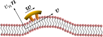
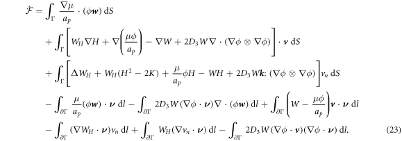
Figure 1. The state of the system, given by the shape of the bilayer mid-surface and by the protein area fraction, can evolve as a result of the membrane velocity ( ), tangential (
 ) and normal (vn), and of the diffusive velocity of proteins relative to the membrane (
 ).
).
Download figure:
Standard image High-resolution image3. Energetics, dissipation and power input
To describe the dynamics of protein-membrane interactions, we adopt a nonlinear Onsager's formalism of dissipative dynamics [57–59], according to which the time evolution of the system follows a minimization principle where energy release and dissipation compete. This nonlinear variational principle is useful to formulate complex models in a very transparent way, and has been invoked in a variety of contexts including low Reynolds number interfacial hydrodynamics [60–62], materials modeling [63–65], soft matter physics in general [66], and membranes in particular [53, 67, 68]. In the present context, the state variables  and ϕ determine the elastic energy (associated to bending) and the chemical energy (entropy and self-interactions) of the system, whereas the variables characterizing changes in the state of the system, here
  and
and  , determine energy dissipation through shear viscous forces in the membrane and friction as proteins move relative to the membrane. Onsager's formalism provides a transparent method to derive the governing equations even in the presence of strong nonlinearity, here caused mechanically by the very large deformations of the membrane and chemically by molecular crowding in protein-rich domains.
3.1. Energetics
To describe the bending energy of the membrane, we follow a classical Helfrich model [36, 37, 69], ignoring the Gaussian curvature terms for simplicity but including a spontaneous curvature that depends on protein density. Assuming a linear dependence of preferred curvature on protein density, a common form of the bending energy is

where κ is the bending modulus and  encodes the curving strength of proteins. Other variants of this model have been proposed [40] and further discussed in section 7.
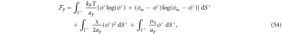
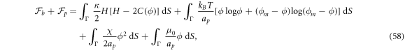
For the free energy of the proteins on the surface, we adopt a Flory–Huggins [38, 39] model accounting for the entropy of mixing and for protein–protein interactions

In this equation,  is the thermal energy, ap is the area on the membrane of a single protein so that ϕ/ap is the number density, the term involving ϕm (a saturation area fraction) accounts for the entropy of uncovered spaces, χ determines the strength and sign (attractive or repulsive) of protein–protein interactions, and μ0 is a reference chemical potential. Variants of this model have been used to understand the linear stability of fully mixed states [42, 43] or to examine protein sorting by curvature at fixed shape [18, 44, 47].
Depending on the parameters and the boundary conditions, the model can lead to phase separation. For instance, negative χ promotes demixing and coexistence of a protein-rich and depleted phases. To regularize phase boundaries, we consider a term penalizing the gradient, which can be interpreted as a non-local interaction of proteins

Λ being a material parameter. The length scale of this interaction is of the order  , which, for a planar membrane, determines the thickness of the interface between protein-rich and depleted domains. Without this term, there is no energetic penalty to domain boundaries and the equations may become ill-posed [70]. Total free energy of this system is then given by

where W represents the total energy density of the membrane-protein composite system. We note that this form of energy density is not the most general that can be conceived for diffusing proteins on an inextensible fluid membrane without orientational order. For instance, the energy could also depend on the scalar invariant  [71].
[71].
A central thermodynamic quantity that drives protein diffusion and sorption is the chemical potential μ [59], measuring the amount of work required to add a molecule at a particular membrane location. The chemical potential can be identified from the variational derivative of  with respect to ϕ as

where  denotes the partial derivative of W with respect to its ith argument. Because this variation is taken at fixed shape,
  . Using the notation
  , and
, and  , and integrating by parts, we obtain

with  representing the in-plane normal at the edge ∂Γ. Ignoring the boundary term, comparison of the two equations above allows us to identify the chemical potential from equation (9) as,

where Δ denotes the surface Laplacian. This expression clearly shows the contributions to the chemical potential given by bending elasticity, entropy and protein self-interactions.
3.2. Dissipation
Having described the mechanisms through which membrane and proteins store energy, we now detail the dynamical modes through which the system dissipates energy. Lipid bilayers in a fluid phase behave like interfacial viscous Newtonian fluids [67, 72]. Here, we ignore dissipative forces resulting from inter-monolayer slippage [52, 53, 73]. Having assumed that the membrane is locally inextensible,  , the dissipation potential accounting for in-plane shear can be written as

where η is the in-plane shear viscosity of the membrane and the rate-of-deformation tensor  is given by equation (2) [67].
Protein transport is characterized by the collective protein velocity  relative to the lipids in the membrane, which has already appeared in the statement of balance of proteins, see equation (5). As a single protein moves relative to the lipids, it experiences a drag force given by
  , where ξ is the molecular drag coefficient. By superposition in a dilute approximation, a collection of proteins characterized by local number density ϕ/ap experiences a drag force per unit area given by
  . The associated dissipation potential can then be written as

For simplicity, we ignore the dissipation occurring in the bulk fluid. This approximation could break down if fast shape changes occurred over length-scales larger than the Saffman–Dellbrück length, of about 1–10 µm [67, 74]. In most situations, however, fast curvature generation by proteins leads to much smaller geometric features [19, 75, 76]. Thus, the total dissipation potential of the system is given by:

3.3. Power input
Let us consider a membrane patch Γ, possibly with smooth boundary ∂Γ. In absence of body forces or sorption of proteins from the bulk, power can only be supplied to the system through edge tractions, moments or flux of proteins at a given chemical potential. Assuming that Γ is a material surface, and thus no lipids can flow through ∂Γ, we write the power input functional as

where μb is a fixed chemical potential for proteins at the boundary, e.g. maintained by a protein reservoir,  is a unit tangent vector along ∂Γ so that
  , Fν and Fn are traction components at the boundary, M is a bending moment per unit length, and
  represents the material time derivative of the surface normal. We can express the last integral in terms of our dynamical variables
  and vn using the relation

where  is the geodesic torsion of the boundary curve and
  its normal curvature [77, 78]. Each of these terms can be defined on Neumann parts of the boundary ∂Γ.
4. Governing equations
4.1. Onsager's variational principle
Onsager's recipe to derive the dissipative dynamics is to minimize the Rayleghian functional defined as

where  is the rate of change of the energy [58, 59]. To enforce local inextensibility, see equation (4), and possibly the incompressibility of the fluid enclosed by the membrane, we introduce a Lagrange multiplier field σ (contributing to membrane tension) and a Lagrange multiplier p (pressure difference) to form the Lagrangian

Since Γ is a material surface, the rate of change of energy can be written as

where  is the material time-derivative of the energy density and is given by

Note carefully that, because  with
with  involves the inverse of the metric tensor, which depends on the membrane configuration, the time derivative in the last term involves not only
  but also the velocity of the surface. Indeed,

Using the above equation, the relation  [67], balance of mass of proteins in equation (5) and the divergence theorem, we can express the rate of change of the energy by explicitly highlighting its dependence on the variables
  and
and 
In the literature dealing with the Cahn–Hilliard equation, related to our model, the second term in the fourth line is set to zero by requiring the natural high-order boundary condition  on ∂Γ [79]. As a result, the last integral over the edge also vanishes. Similarly, we can express the constraint of local area conservation as

To obtain the governing equations of the system, we substitute the above relations in equation (19), minimize the Lagrangian with respect to  and maximize it with respect to {σ, p}. Surface integrals in the two expressions above contribute to the Euler–Lagrange governing equations whereas boundary terms identify the Neumann boundary conditions. The resulting equations for the specific choice of W given in section 3.1 are discussed below.
4.2. Transport of proteins
Minimizing the Lagrangian with respect to the diffusive velocity,  , we obtain the diffusive flux of membrane proteins consistent with Fick's law

Substituting the above relation in equation (5) and using the inextensibility of the lipid membrane we obtain

which can be expanded recalling equation (12) and rearranged to yield the transport equation for proteins

where we have defined the effective interaction between proteins as  . For vanishing spontaneous curvature (
 ), this governing equation ceases to depend explicitly on the curvature of the underlying surface, although it does depend on its geometry through the covariant derivative, and it reduces to a nonlinear Cahn–Hilliard equation [80] on the surface with a density-dependent diffusion coefficient

For χ = 0, Λ = 0 and ϕ ≪ ϕm, equation (27) reduces to the linear diffusion equation. For  , the curvature gradient introduces a bias in the diffusion with drift velocity

driving curved proteins along or against the curvature gradient depending on the sign of  . At steady state, drift and diffusive transport must balance and yield a divergence-free flux.
4.3. In-plane force balance
Minimization of the Lagrangian respect to the in-plane velocity,  , yields

where the first term accounts for the tension required to impose lipid membrane inextensibility, the second term is a force density on the fluid membrane resulting from the relative motion of proteins, see equation (25), and the third term represents tangential dissipative forces due to membrane viscosity, which strongly depend on curvature and involve both tangential and normal velocities as discussed in detail elsewhere [67, 81].
In the common situation of an incompressible Stokes flow with a dilute diffusing species, the drag force density due to protein motion, the second term in equation (30), does not contribute to the hydrodynamics because ϕ∇μ can be expressed as a gradient and grouped with the Lagrange multiplier enforcing incompressibility in all the governing equations [59]. Here, however, this is not the case. Indeed, introducing equation (12) into (30) we obtain

where  is the deviatoric component of this rank-one tensor, and we identify the effective membrane tension (the hydrostatic part of the stress tensor) as

Since the third term in equation (31) cannot be expressed as a gradient, the drift contribution to protein transport generates a tangential force density introducing an explicit coupling between hydrodynamics and protein transport. This protein-induced force just requires the presence of curved proteins and a curvature gradient and can drive flows out-of-equilibrium. Furthermore, as a result of the fundamental in-plane/out-of-plane coupling mediated by curvature [81], this force density can induce out-of-plane forces and shape changes. At steady state, since  is in general different from zero, equation (31) shows that we can expect a non-uniform effective membrane tension in the presence of gradients of curvature. The second term in equation (31) further contributes to a non-uniform and also non-hydrostatic membrane tension in equilibrium, in this case associated to gradients in ϕ.
Going back to the notion of effective tension σeff, one way to think about it is just as a Lagrange multiplier enforcing local inextensibility. However, equation (32) provides further insight about this tension. The first term, σ can be interpreted as the membrane tension of the lipids. The second term is the osmotic tension due to the presence of proteins. In the limit ϕ ≪ ϕm, this term becomes  , recovering the Van't Hoff's equation. The third term accounts for the fact that attractive/repulsive proteins increase/decrease surface tension. The last term is a non-local tension that can become significant at phase boundaries. Thus, σeff is a measure of tension in the composite membrane-protein system. We refer to appendix A for a complementary and detailed derivation of the stress in the present theory.
4.4. Force balance normal to the surface
Minimization with respect to the normal component of the velocity,  , yields

where the first term corresponds to an out-of-plane force density due to membrane curvature elasticity, and hence coupled to the protein density, the second to fourth terms account for Laplace's law, and the last term is a normal viscous force density due to membrane shear, studied in detail in [67, 81].
4.5. Boundary conditions
In the chemo-mechanical problem studied here, we can impose Dirichlet boundary conditions in part of the boundary ∂Γ for the different fields. For instance, reasonable Dirichlet conditions for the mechanical part of the problem include fixing  and
and  on a part of ∂ Γ, where
  and
and  are Dirichlet data. For the chemical problem, the Dirichlet boundary condition is prescribing
  on part of ∂Γ.
On parts of the boundary where Dirichlet boundary conditions are not specified, we obtain the following Neumann boundary conditions by extremizing the Lagrangian and collecting terms at the boundary:

The first condition sets the chemical potential in the Neumann part of the boundary, whereas the next four equations set the applied torque and force per unit length. The in-plane force can be further recast in a form clearly showing the contributions of the effective surface tension and bending energy as

For surfaces at equilibrium with flat boundaries, the forces normal to the boundary per unit length transmitted by the membrane is tangential and given by σeff.
4.6. Time-scales of shape and protein density relaxation
The chemo-mechanical model described by the transport equation for proteins (27), membrane inextensibility (4), force balance in-plane (31) and out-of-plane (33) exhibits multiple intrinsic relaxation time-scales. To examine the competition of mechanical and chemical relaxation time-scales, we consider the simplest cases of shape disturbances whose relaxation is driven by bending elasticity and dragged by membrane viscosity, and of protein density disturbances entropically penalized and dragged by the friction between proteins and the lipid membrane. Such mechanical relaxation occurs during the characteristic time τm = ηℓ2/κ , where ℓis the characteristic size of the disturbance. The characteristic time for protein diffusion is  . Their ratio is thus

where we have used the common estimate for the bending stiffness  . In turn, ξ is related to the membrane surface viscosity η through the Saffman–Delbrück theory [82], which states that

where Lsd ≈ 5 μm is the ratio of membrane and bulk viscosity, ℓa ≈ 1 nm is the effective radius of the protein and γ ≈ 0.577 is the Euler Mascheroni constant. Using this estimation we obtain, ξ ≈ 2πη, which results in  . Thus, mechanical relaxation occurs nearly two orders of magnitude faster than protein relaxation by diffusion. Although other phenomena accounted for in our general theory (such as protein self-interaction, drift by curvature gradients, or mechanical forces due to the presence of curved proteins on the membrane) can influence the dynamics of the system, this simple estimate establishes that in general protein transport can be expected to be the slow process.
5. Axisymmetric formulation and numerical approximation
Under the assumption of axisymmetry, pertinent to many structures resulting from protein-membrane interactions, the shape of the membrane can be parametrized in terms of the distance to the z axis and the z coordinate of its generating curve (ρ(u, t), z(u, t)), where u is a Lagrangian coordinate labeling material particles in the interval [0, 1] and t is time. Protein area fraction does not depend on the azimuthal angle and thus can be expressed as ϕ(u, t). For closed surfaces, smoothness of the surface at the poles is guaranteed by the conditions  and
and  , where
  denotes the partial derivative with respect to u. For an open patch, we replace the condition at u = 1 by
  . The diffusive protein velocity can be expressed as
  , where
  is the unit tangent vector to the generating curve and
  is the speed of this curve.
From the generating curve, we can compute the mean curvature of the surface as

where  [74]. Noting that the element of area is
  , this expression allows us to compute the bending energy
 ![${{ \mathcal F }}_{b}[\rho ,z;\phi ]$](https://content.cld.iop.org/journals/1367-2630/21/9/093004/revision2/njpab3ad6ieqn81.gif) in equation (6).
in equation (6).
As a reference surface  with local radius
  and speed
  is mapped to the current surface Γ with radius ρ and speed a, the local areal stretch at each point is
  . Thus, membrane inextensibility can be expressed as J = 1, or
  . As shown in [74], the membrane dissipation potential in equation (13) for an axisymmetric inextensible membrane described with Lagrangian coordinates can be expressed as

Balance of mass of proteins in equation (5) for an inextensible membrane can be expressed in the present setting as  . Plugging the expression for
  issued from Onsager's principle, we rewrite equation (27) under axisymmetry as

where

is the surface Laplacian of ϕ.
To perform numerical calculations, we use a Galerkin finite element approach based on a B-Spline approximation of the different fields. We numerically represent the state variables as

where BJ are cubic B-spline basis functions, and 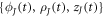 are the Jth control points of the state variables at time t [83]. This approximation provides C2 continuity, enough for our formulation, which requires at least C1 continuity for square integrable curvatures and protein Laplacians.
To move forward in time, we adopt a staggered approach in which we first evolve the protein density field at fixed membrane shape, and then update shape at fixed protein distribution. To obtain the concentration of proteins ϕn+1 at time  , we assume a given shape of membrane {ρn, zn} at time
  , use a backward Euler approximation to discretize equation (40) in time, multiply this equation with a test function ψ(u), integrate over the surface and integrate by parts. For simplicity of our exposition, we assume no flux of proteins through the boundary to obtain
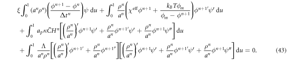
We note that we have further integrated by parts the term involving  to lower the smoothness requirements of the theory. Replacing equation (42) into (43) and choosing the test function ψ = BI, we obtain N discrete equations for ϕJ, I = 1, ... N as

where
Since the matrix KIJ depends on the unknown, the system of equations in equation (44) is nonlinear and we solve it using Newton's method.
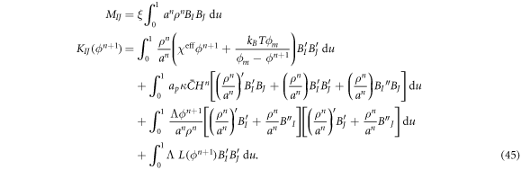
To solve the mechanical problem, we fix protein area fraction to ϕn+1 and write down an incremental Lagrangian accounting for the rate of change of the free energy, for membrane dissipation, and for local area and volume constraints
The Lagrange multiplier  is also discretized in space using B-splines. However, rather than cubic, we use quadratic B-spline basis functions for this field to obtain a stable formulation [84, 85]. To move forward in time, we obtain the mechanical unknown at time tn+1 by numerically solving the algebraic optimization problem

As described above, this Lagrangian method will in general lead to significant distortions of the numerical grid. For robustness and accuracy of the numerical methods, we periodically perform mesh reparametrizations of the generating curve.
6. Results
6.1. Selection of parameters
We choose as the energy scale the bending rigidity of the membrane  . As the length and time-scales, we choose ℓ0 = 50 nm and
  . Considering a membrane viscosity of
  and the relation ξ = 2πη discussed in section 4.6, we obtain that
  , the diffusion coefficient of proteins is
  and τp ≈ 0.02 s. In the absence of measurements, we choose
  large enough so that, when phase separation occurs, domain boundaries have a finite thickness and simulations are devoid of numerical oscillations indicative of ill-conditioning, and small enough so that the dynamics of the problem are not significantly affected by this parameter. With these units, in our calculations we set the non-dimensional coefficients
  (corresponding to
  ),
),  (corresponding to ap ≈ 100 nm2),
  ,
,  and
and  . We finally note that, to avoid numerical solutions with unreasonably thin necks, thinner than the bilayer thickness, we introduce a term that limits the minimum radius of a neck structure to about
  ∼ 7.5 nm by adding an energy contribution of the form

where Γs is the entire surface excluding a small region near the poles and γ = 0.1kBT. We checked that this potential only affected the solutions close to the neck.
6.2. Curvature sensing and generation starting from a prolate vesicle
Curvature sensing is a phenomenon by which curved membrane proteins migrate to regions of the membrane with higher/preferred curvature. Hence, a necessary condition is the existence of a curvature gradient. We first considered a prolate vesicle as shown in figure 2(a). This vesicle is obtained by minimization of bending energy at constant area  , with R0 = 500 nm, at fixed reduced volume v = 0.93. At t = 0, the vesicle is covered with a homogeneous area fraction of curved proteins (
 ) with spontaneous curvature
  . We assume that the proteins are non-interacting and thus choose
  so that χeff = 0. The initial homogeneous distribution of proteins is preferred entropically, but is not optimal from the point of view of bending energy, which favors protein migration towards the poles. The competition between these two free energy contributions leads to a non-uniform chemical potential of proteins and drives protein transport. Since
  at t = 0, protein transport is initially due exclusively to gradients in curvature with the diffusive velocity coinciding with the drift velocity
 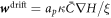 . Estimating the average gradient of mean curvature from the prolate shape, we estimate the time required for drift transport to induce a gradient in protein density as
 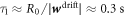 . Subsequently, the dynamics are governed by a competition between drift and diffusive transport, driving proteins towards equilibrium over a time scale
 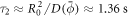 . Thus, we estimate that the total time scale of relaxation is given by τ ≈ τ1 + τ2 ≈ 1.66 s. These estimates are consistent with the results shown in figure 2(a), where we show a few selected snapshots of protein distribution during the equilibration dynamics, along with the time-evolution of the changes in the total energy,
  , and of different components of it. The figure shows that equilibration takes place in a time commensurate to τ, and that protein migration towards the poles is driven by bending energy, which decreases during the dynamics, but opposed by
  . In this example, where the total number of proteins on the membrane is low, their area fraction in the protein-rich poles is far from the saturation area fraction ϕm = 1 and membrane shape does not change.
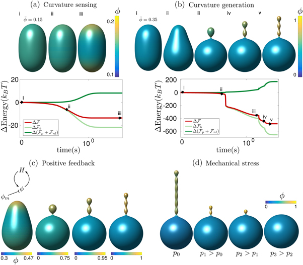
Figure 2. Snapshots of shape and protein coverage during the relaxation dynamics on a prolate membrane vesicle, and time evolution of changes in energies (total, bending and chemical) for an average and initially uniform protein area fraction of (a)  and (b)
  . Supplementary movies 1 and 2, available online at stacks.iop.org/NJP/21/093004/mmedia, show the dynamics in (a) and (b). (c) Final equilibrium states depending on the saturation density ϕm = {0.47, 0.75, 0.95, 1}, which stops the feedback between curvature generation and protein transport. (d) Equilibrium states as vesicle pressure is incremented by steps, while allowing for volume changes, showing a mechanically-induced dissolution of a highly curved and protein-rich membrane domain.
Download figure:
Standard image High-resolution imageTo examine the ability of proteins to generate membrane shape, we revisited the previous example but increased the amount of protein by setting an initial homogeneous area fraction of  , see figure 2(b). At early times, the dynamics parallel those of the previous example, with drift motion of proteins towards the poles, followed by balancing diffusive fluxes. However, now the amount of protein creates a sufficiently large spontaneous curvature
  to modify the shape of the vesicle, which develops a symmetry-breaking transition (ii). At this point, a positive feedback is established during which higher curvature attracts more proteins, which in turn locally increase curvature, and so on. We observe that during this process, the systems develops a cascade of rapid pearling events of duration τm, which create new curvature gradients and thus are followed by the partial equilibration of protein coverage over a time-scale of τp. Similar pearled tubular morphologies have been experimentally and computationally observed in bilayers with isotropic spontaneous curvature caused by anchored polymers [11, 86], in cells as a result of crowding of the grycocalyx [12] or by asymmetric lipid swelling due to changes in pH [87]. We note that if proteins induce anisotropic spontaneous curvature, for instance because they are elongated and adopt nematic order, experiments and molecular models suggest that one can expect tubular protein-rich protrusions of uniform radius [15, 28, 30] rather than pearled protrusions as we find here. We leave models capturing nematic ordering of curved proteins for future work. This pearling cascade and positive feedback loop between curvature and protein coverage continues until proteins almost reach their saturation density ϕm in the highly curved domain. In equilibrium, the system reaches a heterogeneous state where a protein-rich and highly curved pearled tube coexists with a depleted vesicle.
To further examine the role of the saturation area fraction ϕm in setting the equilibrium state, we repeated the previous simulation considering different values of ϕm. Figure 2(c) shows that the depth of the pearling cascade is indeed controlled by this parameter. For ϕm = 0.75, the saturation density and equilibrium is reached after the first pearl has formed. As the saturation area coverage is increased, the number of pearls, and the tube length and curvature progressively increase whereas for lower values of ϕm the system does not even pearl. Thus, in a model governed by the energies in equations (6) and (7), protein saturation controlled by ϕm limits the positive feedback loop between curvature and area coverage.
Curvature generation by membrane proteins involves recruitment of membrane area into protein-rich protrusions, and therefore should depend on membrane tension as shown experimentally [19]. To examine this mechanical coupling, we started from an equilibrium state showing a highly curved protein-rich tube and increased the pressure difference in steps, thus allowing for volume changes in the vesicle. Initially, p0 = 13 Pa and σeff ≈ 0.003 mN m−1. Figure 2(d) shows that as pressure, and thus tension, increase, membrane area is released from the protein-rich tube, which becomes shorter and more concentrated (p1 = 55 Pa, p2 = 65 Pa). Beyond p3 = 250 Pa corresponding to σeff ≈ 0.064 mN m−1, the entire protrusion is eliminated and the proteins uniformly spread over the membrane. This example thus shows the mechanically-induced dissolution of a protein-rich curved domain.
The transition between states of low curvature and homogeneous protein distribution and localized states has been classically analyzed assessing the linear stability of the uniform state [19, 42], summarized in appendix B. According to this analysis, a purely mechanical instability (Euler buckling) takes place when σeff < 0, while a purely chemical instability (phase separation) takes place when  , see equation (28). In addition to these standard instabilities, the system can also exhibit a chemo-mechanical instability involving shape and protein patterning, which in the ideal case of a planar infinite membrane can happen when (appendix B) [19]
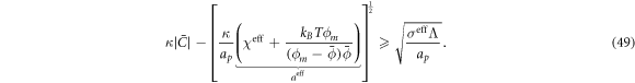
This equation allows us to understand qualitatively the mechanically-induced disappearance of a mechano-chemical pattern as σeff increases in figure 2(d), as well as the emergence of such a pattern when  increases as in figures 2(a) and (b), where χeff = 0.
6.3. Sensing on a tube and shape stabilization
To further study the mechano-chemistry of membrane-protein interactions, we then considered a setup that mimics controlled in vitro experiments, where a curvature gradient is established by pulling a highly curved membrane tether out of a vesicle [16, 18, 44, 88]. We consider the same vesicle size and reduced volume as in the previous examples, and gradually increase the distance between the poles. As in experiments [89], our simulations show that beyond an extension, the system breaks symmetry and a thin tube elongates from one of the poles, see figure 3(a)-i. Starting from this configuration, we load the vesicle with a uniform distribution of proteins with area coverage  . The protein dynamics are similar to the previous examples, with a progressive enrichment of the highly curved tube over a time period of about the diffusive time-scale
 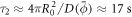 , where now proteins need to migrate a longer distance on average to one of the two poles, figure 3(c). At equilibrium and for this low protein coverage, proteins have barely modified the shape of the vesicle-tube system, figure 3(a)-iii. However, their presence has a noticeable mechanical effect in the force required to keep the tether in place, which decreases by more than two-fold, figure 3(b). This kind of behavior has been experimentally observed for BAR proteins and dynamin [16, 18, 88]. For this protein coverage, however, the amount of protein is insufficient to stabilize the tube and following the release of the displacement constraint, the tube retracts and the protein-rich domain dissolves into the vesicle, figures 3(a)–(c). At higher protein coverage, the proteins drawn to the tube are able to modify visibly its shape by inducing slight pearling, they further reduce the tether force, and the larger protein amount is able to stabilize highly curved and protein-rich protrusions upon release of the constraint, figures 3(d) and (e), in agreement with in vitro experiments [18, 88]. Furthermore, the transition to a strongly pearled protrusion upon force removal (iii–iv) closely mimics the shape transformations in membrane protrusions bent by crowding of the glycocalyx upon disassembly of enclosed actin filaments [12].

Figure 3. (a) Dynamics of curvature sensing by proteins on a vesicle with a tube stabilized by a displacement constraint at a lower average density  . Dynamics of the reaction force (b), average tubular density ϕt and height changes (Δh) (c) before and after the release of the displacement constraint. (d) Evolution of reaction force for higher average densities
  and (e) average tubular density for different average densities showing a density-dependent stabilization of protein-rich curved protrusions. Supplementary movie 3 shows the sensing process and dynamics following constraint release for the lowest and highest average densities.
Download figure:
Standard image High-resolution image6.4. Bud formation and tension-induced dissolution
Buds constitute a prototypical membrane motif, and are involved in endo/exocytosis [2] or in tensional buffering of the plasma membrane through caveolae [4]. Although the formation of such buds requires the synergistic interaction of multiple proteins and lipids, they can be abstracted as curved protein-rich membrane domains [76, 90]. To understand the fundamental mechanism of bud formation, we consider a flat discoidal patch of membrane covered with a homogeneous distribution of proteins ( ) at t = 0. We assume that the membrane is flat at its edge and that proteins cannot flow in or out from the boundary. We apply radial tractions at the boundary corresponding to an isotropic membrane tension of σeff ≈ 3 × 10⁻³ mN m−1, at the lower end of membrane tension in mammalian cells [91].
According to equation (49), the parameters  and aeff/ap ≈ 0.4 mN m−1 should make the initially uniform and flat state unstable, leading to a chemo-mechanical pattern. In agreement with this prediction from the linear stability analysis, our nonlinear, yet axisymmetric, calculations show the spontaneous formation of a budded protein-rich domain as shown in figure 4(a), reminiscent of caveolae. As shown in the figure, this process leads to a significant reduction in the projected area of the membrane patch, and thus during bud formation chemical energy is released to perform mechanical work against the applied tension.
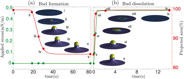
Figure 4. (a) Spontaneous formation of budded protein-rich domain from a flat membrane with homogeneously distributed proteins in the initial state and (b) dissolution of the bud under sudden stress increase, releasing projected membrane area.
Download figure:
Standard image High-resolution imageA critical function of caveolae is the mechano-protection of cells subjected to stretching of the plasma membrane [4]. These budded domains provide a membrane reservoir, which upon tension increase, can be released to buffer membrane tension and avoid lysis [92]. To test the ability of our model to reproduce this phenomenology, we suddenly increased membrane tension to 0.5 mN m−1 within 0.6 s. As a result and in agreement with equation (49), the budded domain rapidly disassembles, leaving a flat patch with uniformly distributed proteins, figure 4(b), consistent with the increased mobility of caveolar components following tension-induced disassembly [4].
7. Two alternative models of membrane-protein interaction
7.1. Proteins with bending elasticity
The curvature model considered up to this point, based on equation (6), assumes that protein cooperativity increases the spontaneous curvature of the surface. However, an alternative model can be conceived in which curved proteins have a stiffness of their own, which results in an effective density-dependent stiffness of the protein shell on the membrane [40]. In this case, the curvature energy of the composite membrane-protein system can be written as

where Cp is the intrinsic curvature of proteins and κp(ϕ) a density-dependent stiffness of the protein coat. The resulting membrane shape is hence the result of the competition between elastic bending energies of proteins and of the lipid bilayer. This model has been used to study the response of membranes with stiff protein coats [93]. Assuming a linear dependence of κp on the protein area fraction,  , and a chemical energy given by equations (7) and (8) as before, the chemical potential of proteins now takes the form

Invoking Onsager's principle with the same dissipation potentials as before, we obtain an alternative protein transport equation

where the density-dependent diffusion coefficient

has the same structure as the one in equation (28). In contrast, the drift velocity  is now qualitatively different, in that its sign relative to ∇H can change in space and time depending on the sign of Cp − H, whereas in the previous model (
 ) it just depended on the sign of the constant
  . Focusing on the case in which both
  and Cp are positive for concreteness, in the model based on equation (6) the drift term always favors protein transport towards regions of higher curvature, whereas in the model based on equation (50) this will be the case only as long as membrane curvature is smaller than the preferred protein curvature. As a result, in the model presented in this section the positive feedback between curvature and protein coverage stops once membrane curvature reaches Cp. Recall that, as discussed in section 6.2, in the previous model this positive feedback was only stopped by the saturation of protein coverage as ϕ approached ϕm. We tested this idea computationally by examining the equilibrium shape predicted by the model based on equation (50) with
  and Cp = 1/25 nm−1, of a slightly deflated vesicle with the same reduced volume v = 0.93 and an average protein concentration
  . Figure 5 shows that the system equilibrates at a state with a protein-rich domain where H ≈ Cp/2 and where ϕ ≈ 0.5 is lower than ϕm = 0.75. The curvature of the protein-rich domain is controlled by the competition of membrane and protein elasticity, which in turn depends on protein coverage. This calculation shows that in this model ϕm does not select the curvature of the protein-rich domain. To further confirm this, we observe that increasing ϕm = 1 does not change the equilibrium state. In contrast, increasing Cp by 17.5% and 20% led to more curved protrusions with a larger number or pearls. Eventually, as protrusions become increasingly concentrated in protein at high values of Cp, protein density reaches saturation and hence ϕm starts playing a role.

Figure 5. Comparison of the equilibrium shapes obtained for different values of the saturation area fraction ϕm and spontaneous curvature Cp for the model governed by the bending energy in equation (50).
Download figure:
Standard image High-resolution image7.2. Membrane bending by protein crowding
Up to this point, we have assumed that proteins interact at the mid-plane of the lipid membrane. However, this approximation clearly breaks down for membrane proteins with bulky partially disordered domains [10, 17] or anchoring long polymers [12]. In this situation, the interaction between proteins leading to bending can be overwhelmingly dominated by the entropic repulsion of these bulky partially disordered domains or polymers, which interact a few nanometers away from the lipid membrane. In the case of polymers attached to a membrane, in addition to their positional entropy, one must account for the changes in conformational entropy of the polymers themselves, which can transition from a mushroom regime to a brush regime as local density increases [12, 33, 94]. Here, we consider the case of proteins with a bulky off-membrane domain, which may be partially disordered but whose conformation does not change significantly with lateral packing. In this situation, we can ignore the entropy of conformational changes of the proteins and their main contribution is due to mixing entropy. Their ability to bend the membrane is related to the fact that curvature modifies the area fraction of proteins at the off-membrane surface where they interact, see figure 6(a).

Figure 6. (a) Illustration of the model accounting for protein crowding of off-membrane bulky domains interacting on a surface  located at a distance d from the bilayer mid-plane Γ. For a fixed number density n on Γ, the figure shows how positive/negative curvature leads to increase/decrease of area fraction of proteins on
  . (b) If proteins are confined to a membrane domain (in red), then an increase in the number of proteins can be accommodated by membrane bending, which reduces the crowding of bulky domains. (c) Equilibrium configurations obtained by increasing the protein average area fraction within a region of constant area. (d) Corresponding jumps in mean curvature as a function of the density dependent spontaneous curvature C(ϕ).
Download figure:
Standard image High-resolution image
Thus, ignoring reconfigurations of the disordered domain/polymer blob [33], we assume that the proteins interact on a surface  at a distance d from the surface representing the lipid membrane, Γ. The free energy of the proteins can then be written as
where  is the area fraction of proteins on
  is the area on this surface of each bulky protein domain, and ϕm is the saturation area fraction of bulky domains on
  .
.
We next refer this energy to the bilayer mid-surface. If the separation between Γ and  is small, dH ≪ 1, then the area element of
  is related to that of Γ according to

Denoting by  the number density of proteins on
  , the above relation shows that we can express the number density on Γ using the relation
  . This relation clearly shows how curvature changes density, as illustrated in figure 6(a) where positive/negative curvature increases/decreases
  at fixed n. Even if the area fraction does not make strict sense on Γ, we can formally define it on the bilayer mid-plane as
  and hence

Denoting by  the diffusive velocity of proteins relative to the bilayer velocity at the membrane mid-plane, protein balance of mass is still given on Γ by equation (5).
Using equations (55) and (56), noting that for small dH we have that  , further assuming that
 ![$\mathrm{log}[{\phi }_{m}-\phi (1-{dH})]\approx \mathrm{log}({\phi }_{m}-\phi )+\phi {dH}/({\phi }_{m}-\phi )$](https://content.cld.iop.org/journals/1367-2630/21/9/093004/revision2/njpab3ad6ieqn150.gif) , which holds true provided that ϕ is not too close to ϕm, and neglecting terms proportional to (dH)2, we can rewrite equation (54) as integral over the lipid surface Γ as
, which holds true provided that ϕ is not too close to ϕm, and neglecting terms proportional to (dH)2, we can rewrite equation (54) as integral over the lipid surface Γ as

Combining this chemical energy with a simple Helfrich energy for the bare bilayer,  , we obtain
where we have defined the protein-induced spontaneous curvature by crowding of off-membrane bulky domains/polymer blobs as

The formal similarity between this expression for  and that obtained in section 3.1 is remarkable, the only difference being that before, the density-dependent spontaneous curvature was simply
  and now it is given by equation (59). Note that the term proportional to
  in the bending energy of the previous model can be dropped by re-defining χ as χeff, and thus it does not affect the structure of the free energy.
In vitro experiments examining membrane bending by protein crowding [10, 17] confined proteins to membrane domains. Not being able to diffuse freely, proteins became increasingly confined, leading to severe membrane remodeling. See figure 6(b). Here, we consider this situation, by allowing ϕ to differ from zero only over a subdomain Γp ⊂ Γ. Over the interface given by ∂ Γp, we thus have an initial jump in protein area fraction of  , the initial average area fraction over the subdomain. Across the interface ∂Γp, forces and moments need to be continuous. Since the energy depends on curvature, jumps in the normal are not allowed but finite jumps in curvature are [69, 95]. Using the expression for the bending moment derived in equation (34) adapted to the free energy density in equation (58), continuity of bending moments across the interface leads to the condition
 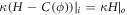 , where the subscripts indicate whether the quantity is evaluated on the inside or on the outside of the interface. We thus conclude that the jump in mean curvature across the interface needs to coincide with the protein-induced spontaneous curvature inside the protein-rich domain,
 ![$[\kern-2pt[ H]\kern-2pt] =C(\phi )$](https://content.cld.iop.org/journals/1367-2630/21/9/093004/revision2/njpab3ad6ieqn157.gif) . To test these ideas, we considered various average protein area fractions,
. To test these ideas, we considered various average protein area fractions, 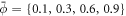 , within a domain of diameter 250nm in a membrane patch of diameter 2.5 μm. We assumed that d = 1 nm and χ/ap = 6 mN m−1 (net repulsive protein–protein interaction). As shown in figure 6(c) increasing the number of proteins leads to increasing curvature, going from very shallow caps to buds, which in all cases very precisely follow the predicted relation for the jump in mean curvature, figure 6(d).
8. Conclusions
We have presented a nonlinear and self-consistent continuum model for the dynamics of membranes interacting with curved proteins. Our theory describes a biologically important instance of chemo-mechanical self-organization leading to surface shape dynamics, which coexists in cells with alternative shape patterning mechanisms [96]. By combining elementary ingredients into a nonlinear Onsager's formalism, we have systematically derived fully nonlinear governing equations exhibiting a tight interplay between geometry, protein transport, and mechanics. Previous simpler models appear as specialized limits of our theory. Our numerical simulations have demonstrated the ability of the model to describe curvature sensing, generation, stabilization, and tension-induced disassembly of protein-rich curved domains. We have developed three versions of the model. We have shown that a common model where spontaneous curvature is proportional to protein density develops a positive feedback between curvature and protein density, only stabilized by protein saturation. An alternative model accounting for the bending elasticity of the protein coat does not exhibit this feature. Finally, a variant of the model where bending is induced by crowding of bulky off-membrane protein domains is formally equivalent to the first model, albeit with a nonlinear relation between protein-induced spontaneous curvature and protein density. The work presented here can be the background for further studies, e.g. accounting for orientational order to model anisotropic proteins such as BAR domains [97], for the interaction of multiple curvature-active species, or developing computational methods to treat the governing equations in 3D [53]. We end by discussing the applicability of the model presented here. While our approach can efficiently treat large numbers of proteins during slow diffusive processes (over minutes and spanning microns), whether continuum models can be quantitative in small systems involving tens of proteins over 10s of nanometers remains to be systematically tested. Furthermore, it is unclear at this moment to what degree the chemical specificity required to understand the biophysics of membrane-protein interactions can be captured by the parameters of our model or variations of it. To address these issues, comparison with coarse-grained molecular dynamics may be particularly interesting, as these models can more easily connect with truly specific atomistic models while accessing larger systems for longer times.
Acknowledgments
We acknowledge the support of the European Research Council (CoG-681434), the European Commission (project H2020-FETPROACT-01-2016-731957), the Spanish Ministry of Economy and Competitiveness/FEDER (BES-2016-078220 to CT), and the Generalitat de Catalunya (SGR-1471, ICREA Academia award to MA).
Appendix A.: Stress vectors
We identify the stress for the membrane-protein system considered here. We first note that, for a surface, stress can expressed in terms of stress vectors with tangential and normal components, 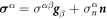 , performing power against
  [77], which can be expressed as

Here, ();α denotes covariant differentiation and (),α partial differentiation. Onsager's formalism naturally allows us to identify each contribution to the stress. For this, we write the Lagrangian in equation (19), ignoring external power input, enclosed volume constraints, freezing protein diffusive transport and assuming for simplicity a closed surface, since our interest here is in the stress, as

where  are the stress vectors associated to the free-energy, dissipation, and inextensibility constraint, and the total stress vector is the sum of these contributions. The expression in the right-hand side leads to the tangential and normal contributions of the stress in the mechanical Euler–Lagrange equation since

We focus first on the free-energy part of the stress and use the fact that for a Lagrangian parametrization  . To identify the stress we assume that proteins do not diffuse, hence the energy only depends on the configuration of the membrane and invoking the chain rule we can write

Since protein transport is frozen for this calculation, W depends on gαβ and kαβ and we have [69, 98]

Using Jacobi's relation, we further have

Substituting the above relation in last term of equation (A.4), we obtain

For the free energy density of the membrane considered here,  , we have

Using  and the relation
  , we obtain

Invoking balance of mass of proteins,  , we have

The equation above can be further used to obtain

The first term in the right-hand side can be further simplified to  by going back to the definition of stress in equation (A.2) and integrating by parts. The derivatives of energy density with respect to second fundamental form are given by

Substituting all the above relations into equation (A.4), we obtain the free-energy contribution to the stress vectors as

Taking the variation of the dissipation potential, a direct calculation allows us to identify  . Similarly, we can identify the component due to inextensibility as
  . These equations above specify the total stress vectors
  for the protein-membrane system. A calculation shows that the tangential and normal components of the equation
  coincide with the tangential and normal statements of force balance in equations (30) and (33).
Appendix B.: Stability analysis
We summarize here the classical linearized stability analysis around a flat square membrane Γ0 of lateral size L covered with homogeneous distribution of proteins with area fraction  . We analyze stability of this homogeneous equilibrium configuration for perturbations in shape and protein density. Placing the flat membrane in the x–y plane and considering shape perturbations described by a Monge parametrization,
 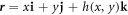 , the areal stretch ratio can be computed as

A perturbation in height of the membrane results in changes in local area and balance of mass of proteins requires that the area fraction of proteins should reduce to  . We consider density perturbations about
  to uncouple them from the perturbations in height. We thus express perturbed area-fractions as

where ϕ is the perturbation.
Expressing the free energy of section 3.1 in the reference configuration Γ0
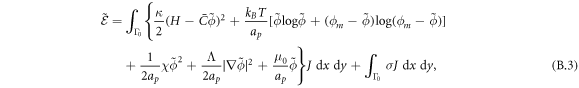
and expanding it up to second order in ϕ and h we obtain

where σeff and aeff are the effective surface tension and self interaction of proteins defined in equations (32) and (49). To evaluate the integral in equation (B.4), we Fourier transform the perturbations to write

for  and
and  where
where  , leading to
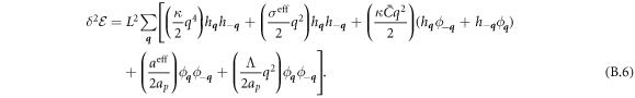
and further to

where  its complex conjugate and
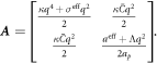
Unstable modes can develop when this matrix ceases to be positive definite. Obvious conditions for instability are σeff < 0 (Euler buckling) and aeff < 0 (purely chemical phase separation). More interesting chemo-mechanical modes of instability develop when both of these quantities are positive but det(A) < 0 or

Since σeff, aeff > 0, for real unstable modes to exist we require that

A similar analysis applies to the free energy discussed in section 7.1, where now
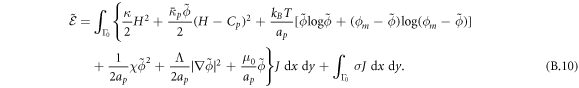
The second variation has the same structure as equation (B.4), the difference being in the interpretation of the coefficients. Now, we have

where
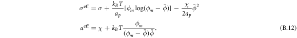
Following the same procedure as before, we obtain the following condition for a chemo-mechanical instability

Qualitatively this condition is similar to that in equation (B.13). However, there is one subtle difference since now aeff and σeff are independent of the spontaneous curvature of the proteins, which was not the case before.