


Abstract
Using the Lanczos recursion method, we exactly determine the shape of the zero-energy Landau level (LL) in a disordered T3 lattice under a strong magnetic field. We discover that the shape of the zero-energy LL depends on the distribution of disorder, but is independent of magnetic field strength. Our analytical study attributes this intriguing behavior to the macroscopic and magnetic field independent degeneracy owing to the existence of the flat band. Moreover, our simulations unravel that the density of states obeys an unconventional scaling law, leading to the fact that the relation between the magnetoconductivity and the carrier density is independent of the disorder strength.
Export citation and abstract BibTeX RIS

Original content from this work may be used under the terms of the Creative Commons Attribution 3.0 licence. Any further distribution of this work must maintain attribution to the author(s) and the title of the work, journal citation and DOI.
1. Introduction
The shape of the Landau levels (LLs) in a disordered two-dimensional electronic system is important to many physical measurements, such as specific heat [1, 2], magnetization [3], magnetocapacitance [4], and magnetoconductivity [5–9]. This subject has been theoretically and experimentally studied for many decades [10–22]. Based on the self-consistent Born approximation (SCBA), the shape of the lowest LL in the conventional two-dimensional electronic systems has been argued to be a semi-elliptical form, which is insensitive to the distribution of disorder [14]. Later, by mapping this problem onto that of a zero-dimensional ϕ4 model, a general nonperturbative approach was proposed to obtain an exact quasi-Gaussian shape for the lowest LL in the presence of the white-noise disorder [11]. After that, a supersymmetry method was extended to discuss the issue in the presence of several different kinds of short-range disorder distributions [12]. It is found that the density of states (DOS) of the lowest LL obeys the following scaling behavior [13]

where B and γ denote the magnetic field strength and disorder distribution variance, respectively. The function form f is closely related to the disorder distribution. Equation (1) also reflects that the width of the LLs Γ depends on both magnetic field strength and disorder strength as  . In our previous studies, we numerically computed the shape of the zero-energy LL in disordered graphene, whose low-energy quasiparticle is governed by the Dirac–Weyl equation with pseudospin-1/2 [18, 19]. Interestingly, our results are similar to the predictions of Wegner in the conventional two-dimensional electron systems.
Recently, there is a growing interest in studying the T3 model [23–33]. Experimentally, the lattice can be realized in a trilayer structure of the face-centered cubic lattice, such as SrTiO3/SrIrO3/SrTiO3 heterostructures [34, 35]. The low-energy quasiparticles of those systems can be well described by the pseudospin-1 Dirac–Weyl equation, predicting the existence of the flat band in their electronic structures. Such a special spectrum leads to distinctive features, such as super-Klein tunneling [29, 32], diverging dc conductivity [30], and anomalous Anderson localization [36]. A natural question arises as to how such a special spectrum affects the shape of the zero-energy LL with disorders. We notice that the disorder effect in the T3 lattice has been discussed by Vidal et al in the large-flux limit (∼h/e) [37]. However, the study in the opposite small-flux limit (∼0.001h/e) is still lacking. In this case, the magnetic field is still strong because of the small lattice spacing.
In this work, using the Lanczos recursion method, we numerically determine the exact DOS of the T3 lattice under a strong magnetic field with the short-range disorder. To illuminate the effect of the disorder on the shape of the LLs, we perform extensive simulations for two different types of disorders: the Gaussian random potential and the Anderson-type uniform random potential [38, 39]. Remarkably, our simulations show that the DOS of the zero-energy LL obeys a scaling law, which is similar to equation (1) but independent of the magnetic field. Concretely, the shape of the zero-energy LL under the Gaussian disorder can be well fitted by the Gaussian function, while that under the uniform distribution is approximately described by a semi-elliptical form. We also present an analytical study to compute the DOS of zero-energy LL based on the SCBA. As a result, we find that the magnetic field independent scaling behavior can be attributed to the magnetic field independent macroscopic degeneracy of the zero-energy LL. Moreover, to demonstrate the significance of the shape of the LLs, the magnetoconductivity is calculated using the linear-response formula [40]. It is shown that the shape of the LLs plays an important role in the transport properties, and the above scaling behavior leads to an interesting fact that the magnetoconductivity as a function of carrier density is independent of the disorder strength. In addition, the existence of the huge magnetic field independent macroscopic degeneracy of zero-energy LL results in blue shifts of the conduction and valence bands LLs, in contrast with what found in the disordered graphene [18, 19].
This paper is structured as follows. In section 2 the tight-binding Hamiltonian and low-energy effective Hamiltonian of the T3 model is specified, the simulation method and parameters are given, and then the calculated results of magnetoconductivity using the linear-response formula are presented. In section 3, we discuss the DOS of the zero-energy LL from our simulations, where the scaling law is proved within numerical accuracy. Finally, we summarize our main outcomes in section 4.
2. The model and methods
2.1. Tight-binding model and simulation method
The geometry of the T3 lattice resembles the honeycomb lattice and accordingly graphene, but with an additional atom that sits at the center of each hexagon, as shown in figure 1(a). Two of these sites are threefold coordinated, denoted by A and B respectively, while the third site is connected to six nearest neighbors (denoted by H) [24]. The nearest-neighbor hopping takes place between sites A, B, and H with strength  , while the hopping between sites A and B is forbidden. Thus the T3 lattice is bipartite and particle-hole symmetric [28]. The tight-binding Hamiltonian can be written as

where cAi, cBi and cHi denotes the annihilation operator for a particle of unit cell i on site A, B and H, respectively.

Figure 1. (a) The geometry of the T3 lattice. The honeycomb unit cell with the three sublattice A (red circles), B (green circles), and H (black circles) is indicated, where lines denote the nearest-neighbor hopping and a is the lattice constant. (b) Zero field energy spectrum as a function of the wave vector.
Download figure:
Standard image High-resolution imageThe short-range disorder potential is modeled by random on-site energy

where  's are random variables and the disorder is assumed to be uncorrelated, that is,
  . In this work, two probability distributions of on-site energy are considered: the Gaussian distribution with standard derivation σ and the uniform distribution with an interval [−W/2, W/2]. Their variances γ equal to σ2 and W2/12, respectively. The applied perpendicular magnetic field B = (0, 0, B) and the Landau gauge is chosen as A = (0, Bx, 0) in our simulations. In the tight-binding model, the magnetic field can be introduced via Peierls substitution: the hopping term t is multiplied by a phase factor
  involving the vector potential A

where the integration path is the shortest distance over the nearest neighbor bond from site m to site n.
The DOS is calculated with the Lanczos recursion method [18, 19]. The averaged DOS can be evaluated from the Green's function

The small artificial cutoff energy η is chosen as η = 10−3t, which is rather smaller than the broadening of the LLs investigated. The random phase state is used to reduce the time complexity [41]. The random phase state is defined through

where N denotes the total number of sites and {θn} are a set of independent random variables uniformly distributed on [0, 2π]. Because of the large systems and weak disorder considered in this work, one or few different random phase states is sufficient to obtain a good estimation of the averaged DOS.
In our simulations, the shape of the finite cluster is diamond as shown in figure 1 (a) and the periodic boundary condition is imposed. The cluster comprises Ω/A = 40002 unit cells in this work, where Ω is the area of the system,  denotes unit cell area, and a is the lattice constant as shown in figure 1(a). For simplicity, we define a unit magnetic field strength as
  , i.e. the magnetic flux threading through per unit cell
  in our simulations. If using the lattice constant of graphene a = 2.47 Å, we obtain B0 ∼ 50T which is accessible experimentally. All calculations are carried out on a 2.00 GHz Xeon 3 CPU work station, and each simulation for a single realization of a random phase state under specific disorder realization requires around 20 h of computing time running on 32 cores.
2.2. Low-energy effective Hamiltonian and LLs
In the absence of the magnetic field, the energy spectrum of the T3 lattice is plotted in figure 1(b), which contains three branches, including two electron–hole symmetric conduction and valence bands, and a unique flat band at the charge neutrality point. The dispersion of conduction and valence bands are identical to the bands in graphene and features two inequivalent Dirac cones.
In the presence of the magnetic field, here, we employ its effective Hamiltonian obtained by a long-wavelength approximation from the tight-binding Hamiltonian to describe the low-energy properties. For a given Dirac point, the Hamiltonian reads

where  is the Fermi velocity, k = (kx, ky) is the momentum operator, and S denotes the pseudospin

Combining with

Sx, Sy form a 3-dimensional representation of SU(2), satisfying commutation relation [Si, Sj] = iijkSk, similar to the Pauli matrix. Although they have higher pseudospin, they can not form a Clifford algebra {Si, Sj}  2δij [29].
The corresponding LLs energies are expressed as

where  is the magnetic length, s = ± denotes the conduction band and valence band respectively with the LL index n = 1, 2, ..., and s = 0 labels the LL at zero energy with index n = 0, 2, 3, ...[29, 42, 43]. The total number of the Landau indexes NΦ for each band is determined by the semiclassical quantization rule [44]

where the factor 2 stems from the valley degrees of freedom. Since NΦ is large, we obtain NΦ = πl2/A.
The corresponding eigenfunctions of the low-energy effective Hamiltonian in equation (7) are given by
where ky is the wave number in the y direction, ϕn (n = 0, 1, 2, ...) are eigenfunctions of the one-dimensional harmonic oscillator, and for convenience we set ϕn = 0 if n is negative. Here, parameters Cs, asn, bsn are given by
and

Notice that equations (13)–(14) are well defined only when s = ± with n = 1, 2, ...and s = 0 with n = 0, 2, 3, ..., otherwise, their values are 0. For example, a01 = b01 = 0.
2.3. Magnetoconductivity
To demonstrate significance of the shape of the LLs for physical properties, we calculate the longitudinal magnetoconductivity using the linear-response theory as an example [40]. The magnetoconductivity σyycol is given by

where β = 1/kBT,  is the Fermi–Dirac distribution and Wζζ' is the transition rate in the presence of disorder. The sum is over all quantum number
  and the expectation value of the x coordinate is
  . If the impurity potential is short-ranged, the transition rate is expressed as

Here, the form factor Fζζ' is defined as  .
.
The magnetoconductivity of the LLs with s = ±1 is calculated by Biswas et al [33]. In their work, the scattering between eigenstates is only allowed with identical Landau indexes n = n', because of the existence of the term δ(εζ − εζ') in equation (17). However, this restriction is not valid for the zero-energy LL, and the contribution from the scattering between eigenstates with different Landau indexes must be calculated carefully and integrally.
Using the identity
we obtain the square of form factor for the zero-energy LL
where u = q2l2/2 and Ln(α)'s are generalized Laguerre polynomials. Generally, the disorder scattering gives a finite relaxation time τ, which are ignored in equation (17). A simple and heuristic way to account for this disorder effect is to replace the delta function in equation (17) by a Lorentzian. The relaxation time τ can be estimated from the width of level broadening Γ, τ = ℏ/Γ. Therefore, we replace the delta function by the Lorentzian  [45, 46]. For intra-level scattering, we can further replace the delta function by
  , εζ'/πΓ[33, 8]. As a result of the above, we have

Using the orthogonality of Laguerre polynomials

where Γ(n) denotes the gamma function, and the recurrence relation

we derive

At low temperatures, we can make the approximation ![$\beta {\mathsf{f}}(\varepsilon )\left[1-{\mathsf{f}}(\varepsilon )\right]\approx \delta (\varepsilon -{\varepsilon }_{F})$](https://content.cld.iop.org/journals/1367-2630/21/7/073013/revision2/njpab2bb4ieqn17.gif) . Near the zero energy, the averaged DOS is defined as
. Near the zero energy, the averaged DOS is defined as  in the clean limit, where 2 comes from the valley degeneracy. The energies εζ's in equation (20) are unperturbed eigenvalues calculated in the clean system, which are highly degenerate, especially for the zero-energy LL. However, the disorder scattering will shift the unperturbed eigenvalues and lift the degeneracy. The distribution of the shifted eigenenergies is determined by the DOS. At low temperature, therefore, we can approximately replace the delta function by the numerically calculated DOS in our calculations [47, 33]. Thus the magnetoconductivity can be expressed in terms of the DOS as

where

According to equations (13) and (14), the large NΦ limit of the sum in equation (25) is equal to  . Within this approximation, the magnetoconductivity can be expressed as

3. Results and discussion
Before investigating the simulation results, it is necessary to figure out how many states there are in each LL, in view of the finite system size. For the conduction and valence bands LLs, the degeneracy is determined by the total magnetic flux going through the system, denoted by  , where the prefactor 2 comes from the valley degrees of freedom. Because of the existence of the flat band, the degeneracy of the zero-energy LL is much greater and equals to NΦNk = Ω/A, which is independent of the magnetic field strength.
The DOS of the LLs under Gaussian disorder and the uniform disorder are plotted in figure 2(a). The DOS of the zero-energy LL is much higher and wider than the other LLs since the area of the peak is proportional to the corresponding LL degeneracy. Analogous to the case in graphene, the conduction and valence bands LLs in the T3 lattice are distributed unevenly due to the unique linear dispersion relation. As depicted in figure 2(b), the conduction and valence bands LLs at both sides are pushed away from the zero energy, due to the repulsion from the zero-energy LL. This blue shifts phenomenon is in sharp contrast with the disordered graphene [18]. That is because of the extraordinarily huge degeneracy of the zero-energy LL in the T3 lattice.

Figure 2. (a) The DOS of the T3 lattice under magnetic field B/B0 = 1 with uniform disorder W/t = 0.1 and the Gaussian disorder  respectively. (b) The blue shifts of the conduction and valence LLs of the T3 lattice with uniform disorder W/t = 0.2 under magnetic field B/B0 = 1. The dashed gray lines point out the positions of LLs without disorder in equation (10).
Download figure:
Standard image High-resolution imageNext, we focus on the dependence of the zero-energy LL on the disorder and magnetic field. Due to the magnetic field independent degeneracy, it is expected to exhibit a distinct different scaling behavior from equation (1) [13, 48]. Within the SCBA (see in appendix), we find that the zero-energy LL in the T3 lattice is semi-elliptical:  , which is independent of the magnetic field strength. Compared to equation (1), we propose the following magnetic field independent scaling law to describe the disorder broadened zero-energy LL:

where the form of the function f is closely related to disorder distribution.
In the presence of Gaussian disorder, the scaled numerical calculated DOS  of the zero-energy LL as a function of the scaled energy
  is plotted in figure 3(a). The symbols represent the results for different disorder strengths and magnetic fields. They collapse onto the same curve, well supporting the scaling law in equation (27). Furthermore, the function f with Gaussian disorder can be well fitted by a Gaussian function, which is similar to that in two-dimensional gas and graphene [11, 12, 18]. As for the uniform disorder, the scaling law still holds, although the form of f has changed. In figure 3(b), the shape of the zero-energy LL can be approximately described by a semi-elliptical form derived from SCBA (see appendix for details). Notice that the deviation between our numerical results and the SCBA prediction (especially at E = 0) may come from some nonperturbative effects. In view of the existence of the flat band, the successful nonperturbative supersymmetry method [11, 12] cannot be applied to study the shape of the zero-energy LL directly in our case. This challenging problem is unsolved and needs further investigation.

Figure 3. (a) The scaled DOS of the zero-energy LL with different magnetic fields and Gaussian disorders: B/B0 = 1 and  (red square), B/B0 = 4 and
  (blue circle) and B/B0 = 9 and
  (green triangle). The black solid line represents the Gaussian function fitting curve. (b) The scaled DOS of the zero-energy LL with different magnetic fields and the uniform disorders: B/B0 = 1 and W/t = 0.1 (red square), B/B0 = 4 and W/t = 0.1 (blue circle) and B/B0 = 9 and W/t = 0.2 (green triangle). The black solid line represents the semi-elliptical curve derived from SCBA (equation (A.10) in appendix).
Download figure:
Standard image High-resolution imageTo further check the scaling law, we plot the LL width as a function of disorder strength  in figure 4, since equation (27) indicates that there exists a linear relation between them. The slopes of the fitting curves are 1.96 ± 0.03 and 2.41 ± 0.07 for the Gaussian and the uniform disorder, respectively. Additionally, although the SCBA fails to describe the exact shape of LL, the linear relation between LL width and disorder from SCBA is in good agreement with the numerical results with the uniform disorder:
  .
.
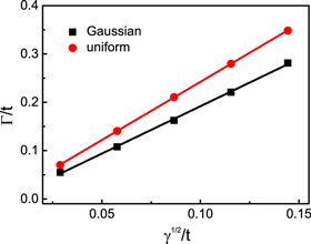
Figure 4. The width of the DOS of flat band LL as a function of disorder strength W under magnetic field B/B0 = 9. The black squares and red circles represent the widths under Gaussian and the uniform disorder of different strengths respectively, and the solid lines represent the linear fitting curves.
Download figure:
Standard image High-resolution imageFinally, as an example of physical measurements related to the DOS of LL, we calculate the longitudinal magnetoconductivity σyycol. The carrier density is defined through

and we can derive it by numerical integration. Substituting the scaling law equation (27) in equation (28), the charge density is expressed as

Using the equations (26) and (28), we calculate the longitudinal magnetoconductivity  as a function of the carrier density ne as plotted in figure 5. Furthermore, by substituting equation (29) into equation (26), the magnetoconductivity can be written as

Thus, the magnetoconductivity is proportional to B−4 in the T3 model, and this is contrary to the case in graphene, where the longitudinal magnetoconductivity saturates to a value ∼e2/h under high magnetic field [18, 49]. Since the linear relation between LL width and  is independent of disorder strength, equation (30) shows that the magnetoconductivity is independent of disorder strength for fixed carrier density. This conclusion is also well verified by our simulations, as shown in figure 5, where the magnetoconductivities with different disorder strengths collapse onto the same curves.

Figure 5. The magnetoconductivity σyycol versus the carrier density ne at fix magnetic field B/B0 = 9. The black curve and circles represent the magnetoconductivity for Gaussian disorder with the standard derivation  and
and  , and the red curve and circles represent that for the uniform disorder with width W/t = 0.1 and 0.2 respectively.
Download figure:
Standard image High-resolution image
4. Conclusion
In summary, we numerically determine the exact shape of the zero-energy LL in a disordered T3 lattice under strong magnetic field. Because of the small lattice spacing, although the magnetic flux per unit cell is small, the magnetic field is large and strong enough to avoid the mixing of disorder broadened LLs. We confirm that the existence of the flat band in the T3 model leads to magnetic field independent scaling behavior of the zero-energy LL, in sharp contrast with graphene. Such unconventional scaling behavior results in the interesting fact that the magnetoconductivity is proportional to 1/B4. Since the T3 model may be realized in electronic materials and cold-atom systems [34, 35, 26], we believe our predictions can be tested by thermodynamics and transport measurements in experiments.
Acknowledgments
This work was partially supported by National Key Research & Development Program of China (No. 2016YFA0200604 and 2017YFA0204904), and by the National Natural Science Foundation of China (Nos. 11874337, 11634011, and 21873088). Computational resources are provided by the Chinese Academy of Sciences, Shanghai and USTC Supercomputer Centers.
: Appendix. Self-consistent Born approximation
To understand the unconventional scaling behavior above, we calculate the DOS of zero-energy LL within SCBA [14]. Since the energy spacing between the LLs with different band indexes s is large enough, the contribution to the self-energy from weak disorder scattering between different band indexes s is negligible. Because the translational invariance is recovered after impurity averaging, the self-energy becomes diagonal with respect to the wave factor ky. The diagonality with respect to LL index n can be obtained as below. The first order of self-energy is given by

where  . Here the disorder is short ranged
  , where γ = W2/12 for the uniform disorder and γ = σ2 for the Gaussian disorder. After some algebra, we obtain

where  . Therefore the first order of self-energy is diagonal with respect to s, n, ky. Using the recursion relation of the self-energy

and the diagonality of G0 with respect to s, n, ky, we can generalized the diagonality in equation (A.1) to arbitrary order of the self-energy. In the end, the self-energy within SCBA takes the form

thus the Green function is also diagonal

After some algebra, the impurity averaged Green's function and self-energy can be written as

Notice that Σ+n is identical to Σ−n explicitly because a−n = a+n, and b−n = b+n, since the electron–hole symmetry is retained.
Generally, equation (A.6) can be solved numerically, while the analytical treatment need some approximation. For the zero-energy LL in the large LL index limit, we obtain

where the valley degree of freedom has been taken into account in terms of the number Nk. It will be a proper approximation to keep G0n only since the LL mixing can be neglected in a strong magnetic field and the contribution from the zero-energy LL is dominant [50]. Furthermore, in view of the macroscopic degeneracy of the zero-energy LL, the self-energy dependence of the zero-energy LL upon the Landau index n can be ignored, so that Σ0n ≈ Σ0 and G0n ≈ G0 and the sum over LL indexes equals NΦ. All in all, we obtain

Notice that disorder strength is the only surviving physical parameter, thus the DOS is expected to be independent of magnetic field. The analytical solution of the zero-energy LL is

and the DOS is expressed as

In conclusion, a semi-elliptical DOS of the zero-energy LL is suggested within SCBA no matter what kind of disorder distribution is considered. On the other hand, equation (A.10) gives a linear relation between LL width and disorder  .
.