Latent heat of traffic moving from rest

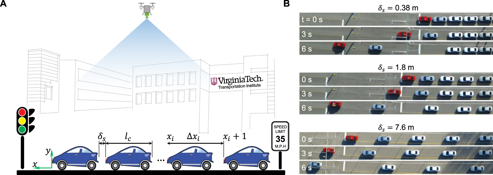
Ten volunteer drivers conducted a study on the closed-circuit Smart Road located at the Virginia Tech Transportation Institute (figure 1(A)). Each driver was provided a Chevy Impala (LS Sedan 4D, 2011-2012) of identical dimensions that was rented from Virginia Tech Fleet Services and insured for the study. The Smart Road includes a traffic light located in the middle of a flat, straight road with single lanes and a speed limit of 35 mph (15.6 m s⁻¹). The traffic light was initially set to red and all ten volunteer drivers were instructed to line up in a queue. Using radio transmitters and approved safety protocols (IRB #15-484, see appendix A), each driver came to a stop at a fixed bumper-to-bumper spacing (${\delta }_{s}$) from the car ahead. Spacings were measured by fixing a tape measure between two tall traffic cones; one cone was placed at the rear bumper of a car already stopped in 'Park', while another car was instructed to slowly approach the second cone until its front bumper made contact. For any given trial, all cars in the queue exhibited an identical value of ${\delta }_{s}$, which was varied to be either 1.25 ft (0.38 m), 3 ft (0.91 m), 6 ft (1.8 m), 12 ft (3.6 m), 25 ft (7.6 m), or 50 ft (15 m). Once all ten cars were queued at the red light with the appropriate spacing, a drone helicopter (DJI Inspire 1) was programmed to hover over the intersection at a fixed elevation of 200 ft (61 m) with respect to the road. The drone included a digital video camera attached to a gimbal (DJI Zenmuse X3) to obtain controlled bird's-eye-view footage of the traffic. All drivers could see the traffic signal and they were instructed to accelerate in a normal and comfortable fashion up to the road's speed limit of 35 mph when the light turned green. It was strongly emphasized that the bumper-to-bumper spacing initially imposed at the red light does not need to be maintained once flow resumed. Three trials were captured for each car spacing, with the order of the drivers changing for each trial. For consistency, the three different driver orders chosen for the three trials were kept the same for all six car spacings. When the cars and drone were all in place, the drivers were instructed to put their cars in 'Drive' and proceed through the intersection when the light turned green. Once all drivers confirmed via radio that they were idling and ready to go, the traffic light was turned to green using a Smart phone interfaced with the Smart light.

Zoom In Zoom Out Reset image size

The drone footage showed that it takes more time for cars to begin to accelerate with decreasing ${\delta }_{s}$ (figure 1(B)). For example, when ${\delta }_{s}=0.38\,$ m (top images), the third car in the queue is not moving even after 6 s from when the first car began to accelerate through the intersection. This is because of the long delay time required for each car to regain a safe distance to the car ahead before readily accelerating (latent heat). In contrast, when ${\delta }_{s}=7.6$ m, the latent heat is reduced and even the fifth car is able to move within the initial 6 s.

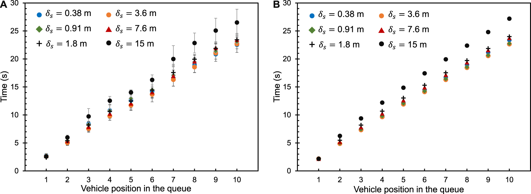
An open-source software (Tracker) was used to convert the drone footage to displacement plots for each car. Solid lines in figure 2 show the displacements of the front bumpers of all ten cars over time for each value of ${\delta }_{s}$, with all values being averaged from the 3 separate trials to mitigate effects of driver variability. Remarkably, the time required for all ten cars to cross the intersection remained fixed at 23.0  ±  1.1 s for all spacings ranging from ${\delta }_{s}=0.38$ m up to ${\delta }_{s}=7.6$ m (figure 3(A)), even though in the latter case ${\delta }_{s}$ is larger by a factor of 20 and the vehicles are traveling twice as far to cross the intersection (figure 2(A), (E)). This balance between reduced lag and increased displacement is eventually lost, but only for the extreme case where ${\delta }_{s}$ exceeds the minimum spacing required for comfortable driving (analogous to a 'gas phase'). For example, the cars required a slightly larger time of 27  ±  3 s for ${\delta }_{s}=15$ m (figure 3(A)). Moreover, as it is depicted in figure C1(A), the time required for each car to cross the intersection was found independent of the static bumper-to-bumper spacing as ${\delta }_{s}$ varies from 0.38 to 7.6 m.

Zoom In Zoom Out Reset image size

Zoom In Zoom Out Reset image size

Zoom In Zoom Out Reset image size

It is already well known that the saturation flow rate of vehicles passing through a green light is generally fixed around 1500–1800 vphg (vehicles per hour of green) over a wide variety of natural driving conditions [42–44]. However, this is because the saturation flow rate only considers the steady-state case of cars that are already crossing the intersection with a constant liquid-phase headway (figure C2(A)) [45–47], thus ignoring the initial start-up lost time where the solid-to-liquid transition actually occurs. Our focus here is therefore not on the saturation flow rate, but on the start-up lost time (i.e. departure flow rate) which considers the time required for the first four cars in the queue to cross the intersection when the light first turns green. By breaking up the total time required for all 10 cars to cross the intersection into the transient and steady times, we observe that both the departure flow rate and the saturation flow rate are insensitive to ${\delta }_{s}$ for all solid and liquid-phase packing densities (figures 3(A), C2(B)). By definition, it is obvious that the saturation flow rate is independent of ${\delta }_{s}$, so we emphasize that our surprising finding is that even the start-up lost time is invariant with ${\delta }_{s}$ due to the effect of latent heat. Previous reports have characterized how the start-up lost time can be affected by inclement weather [48], countdown timers [49, 50], the time of day or speed limit [51], and distracted drivers [52, 53]. However, to our knowledge there are no reports where the effects of the initial (static) car spacing on the start-up lost time were investigated, which is the novelty of our present work.

The above results show the pronounced effect of latent heat on group motion from rest, which will now be examined analytically using the OVM. The development of a theoretical model will be especially useful for extrapolating the displacement curves of the experiments done with large spacings (${\delta }_{s}\geqslant 3.6$ m), where the drone's field-of-view could not capture the initial position and acceleration of several cars at the back of the queue (see figures 2(D)–(F) and movie S2). Recall that the OVM is a semi-empirical microscopic model and can be used to develop theoretical displacement curves to match the experiments. The equation of motion for the i-th car with mass M and velocity v_i is [32]:

$$\begin{eqnarray}&&M\displaystyle \frac{{{\rm{d}}{v}}_{i}}{{\rm{d}}{t}}={F}_{\mathrm{acc}}({v}_{i})+{F}_{\mathrm{dec}}({\rm{\Delta }}{x}_{i}),\end{eqnarray} \tag{ 1 }$$

where ${F}_{\mathrm{acc}}$ and ${F}_{\mathrm{dec}}$ are the acceleration and deceleration forces acting on the car, respectively, and ${\rm{\Delta }}{x}_{i}$ is the headway distance between the $(i+1)$th and ith cars (${\rm{\Delta }}{x}_{i}={x}_{i+1}-{x}_{i}$).

The acceleration and deceleration functions are defined as:

$$\begin{eqnarray}&&{F}_{\mathrm{acc}}({v}_{i})=\displaystyle \frac{M}{\tau }({V}_{\max }-{v}_{i})\geqslant 0,\end{eqnarray} \tag{ 2 }$$

$$\begin{eqnarray}&&{F}_{\mathrm{dec}}({\rm{\Delta }}{x}_{i})=\displaystyle \frac{M}{\tau }({V}_{\mathrm{opt}}({\rm{\Delta }}{x}_{i})-{V}_{\max })\leqslant 0,\end{eqnarray} \tag{ 3 }$$

where τ is the delay time and defined as the inverse of drivers' sensitivity ($\tau =1/a$). The higher the sensitivity of a driver, the faster the driver will accelerate or decelerate to reach the optimal velocity. The value of a is typically chosen to fit the model to the experimental displacement curves; here, a constant value of a = 0.15 s⁻¹ was assigned to all drivers. The V_max term in equation (2) corresponds to the speed limit of the road (15.6 m s⁻¹). In equation (3), ${V}_{\mathrm{opt}}({\rm{\Delta }}{x}_{i})$ represents the optimal velocity desired by each car at any moment in time as a function of the headway distance, and is represented by the optimal velocity function (OVF) [16]:

$$\begin{eqnarray}&&{V}_{\mathrm{opt}}({\rm{\Delta }}{x}_{i})={v}_{0}[\tanh (m({\rm{\Delta }}{x}_{i}-{b}_{f}))-\tanh (m({b}_{c}-{b}_{f}))],\end{eqnarray} \tag{ 4 }$$

where the four parameters v₀, m, b_f and b_c are constants obtained from the experiments. Specifically, v₀ is a velocity term solved from boundary conditions, m is a fitting parameter, b_f is the inflection point in the OVF, and b_c is the critical lower limit of the headway distance that represents jamming. Note that while there are alternate expressions for the OVF in the literature [24, 34], we found that equation (4) resulted in the best fit with the experimental data.

To obtain the value of b_c, let us define the actual length of the car as l_c, which is approximately 5 m for the Chevy Impalas used in this study. Obviously, even in traffic jams each driver must maintain a headway distance larger than the actual car length to avoid crashing. Therefore the effective length of each car (b_c) must include a minimal bumper-to-bumper spacing (typically ${\delta }_{j}=2$ m), such that ${b}_{c}={l}_{c}+{\delta }_{j}=7$ m. Note that for the controlled experiments performed here, the parameter space deliberately included ${\delta }_{s}\lt {\delta }_{j}$ (by virtue of using traffic cones and spotters) to probe the full extent of latent heat. A solution for v₀ can be obtained by considering the limiting case of ${\rm{\Delta }}{x}_{i}\to \infty$, where the optimal velocity of each car will simply be the speed limit (${V}_{\mathrm{opt}}(\infty )={V}_{\max }$) and $\tanh (m({\rm{\Delta }}{x}_{i}-{b}_{f}))\to \tanh (\infty )=1$. This simplifies equation (4) to ${v}_{0}={V}_{\max }/[1-\tanh (m({b}_{c}-{b}_{f}))]$, where here $m=2$ m⁻¹ for each spacing. Finally, the inflection point of the OVF is defined as ${b}_{f}={l}_{c}+B$ in which ${V}_{\mathrm{opt}}({b}_{f})={V}_{\max }-{v}_{0}$ and B is a fitting parameter to be determined from the experimental data. In equation (3), the deceleration force reaches to its maximum value when ${V}_{\mathrm{opt}}({b}_{c})=0$ and it goes to zero as ${\rm{\Delta }}{x}_{i}$ goes to infinity. In summary, we utilize a constant value for τ, ${V}_{\max }$, l_c, ${\delta }_{j}$, b_c, and m for all trials, such that only B and by extension b_f and v₀ are varying with ${\delta }_{s}$. For a given trial, all of these terms are the same for all ten drivers. Despite the fact that ${\delta }_{s}\lt {\delta }_{j}$ for some of the experiments here (${\delta }_{s}=0.38$ m and ${\delta }_{s}=0.91$ m), fitting B to the experimental data ensures that ${V}_{\mathrm{opt}}({\rm{\Delta }}{x}_{i})\geqslant 0$ over the entire parameter space even when modeling the initial motion from rest (figure C3).

The governing differential equations of the system can be found by substituting equations (2) and (3) into equation (1) [16]:

$$\begin{eqnarray}&&\displaystyle \frac{{{\rm{d}}{x}}_{i}}{{\rm{d}}{t}}={v}_{i},\end{eqnarray} \tag{ 5 }$$

$$\begin{eqnarray}&&\displaystyle \frac{{{\rm{d}}{v}}_{i}}{{\rm{d}}{t}}=a({V}_{\mathrm{opt}}({\rm{\Delta }}{x}_{i})-{v}_{i}).\end{eqnarray} \tag{ 6 }$$

We have used Mathematica to integrate the coupled equations of motion, equations (5) and (6), in order to determine the position and velocity of each car at every moment of time. The dashed black lines in figure 2 show the theoretical displacement curves, which agree with their experimental counterparts within the experimental uncertainty for all times (figure C4). Therefore, we can use the theoretical solution to extract all of the velocity and acceleration curves for each spacing (figures C5 and C6). Note that minor differences in the initial positions of the cars are due to imperfections in aligning the cars experimentally compared to the perfectly consistent values of ${\delta }_{s}$ used in the model.

By plotting the theoretical displacement curves of the final (tenth) car in the line for each value of ${\delta }_{s}$, it can be seen that the increased travel distance required for liquid phase queues is perfectly compensated for by a reduced lag in acceleration compared to solid phase queues (figure 3(B)). This is also evident by looking at the drone footage for each value of ${\delta }_{s}$ (figure S3 and movie S2). As mentioned before, the time required to clear the intersection does finally increase for the largest ('gas phase') spacing of ${\delta }_{s}=15$ m, where the increase in required displacement finally becomes greater than the reduction in lag. The theoretical time required for each of the ten cars to cross the intersection is in excellent agreement with the experimental results (figure C1).

As ${\delta }_{s}$ increases, the delay time required until each vehicle begins to move with respect to the car in front of it will be decreased (figures C5 and C6). For example, 20 s after the first car begins to move, the average velocity of the tenth car increased by 49% when comparing ${\delta }_{s}=0.9$ m to ${\delta }_{s}=7.6$ m.

To characterize the lag of vehicular motion in terms of the concept of latent heat, we first need to develop an expression for the internal energy of the system. The total interaction potential of the vehicles is [34]:

$$\begin{eqnarray}&&U=\sum _{i=1}^{n}\phi ({\rm{\Delta }}{x}_{i}),\end{eqnarray} \tag{ 7 }$$

where $\phi ({\rm{\Delta }}{x}_{i})$ is the interaction potential function which represents the interaction between the $(i+1)$th car and the ith car ahead. The interaction potential function can be obtained from the integration of the deceleration force function with respect to ${\rm{\Delta }}{x}_{i}$:

$$\begin{eqnarray}&&\phi ({\rm{\Delta }}{x}_{i})=\displaystyle \frac{{{MV}}_{{\rm{\max }}}\mathrm{log}(1+{e}^{2m({b}_{f}-{\rm{\Delta }}{x}_{i})})}{\tau m(1-\tanh m({b}_{c}-{b}_{f}))},\end{eqnarray} \tag{ 8 }$$

with the boundary condition $\phi (\infty )=0$ (see the appendi B for the full derivations). Figure 3(D) plots the total non-dimensionalized interaction potential, ${U}^{* }=U/(1/2{{MV}}_{\max }^{2})$, versus time for each value of ${\delta }_{s}$. As expected, the interaction potential of the system is dramatically larger with decreasing ${\delta }_{s}$, for example the potential for ${\delta }_{s}=0.38$ m (smallest spacing) is nearly three times larger than for ${\delta }_{s}=15$ m (biggest spacing). Interestingly, the interaction potential is completely reduced to zero well before the cars are able to cross the intersection, which reveals that drivers do not feel comfortable reaching even moderate velocities under the presence of internal energy. This explains the significant lag time of close-packed queues of vehicles upon resumption of flow, where the interaction potentials are dramatically increased relative to loose-packed systems. We therefore define the latent heat of fusion as equivalent to the queue's total interaction potential at rest. To our knowledge, this is the first such definition of latent heat with regards to group motion from rest.

The total kinetic energy of the system is:

$$\begin{eqnarray}&&K=\sum _{i=1}^{n}\displaystyle \frac{{{Mv}}_{i}^{2}}{2},\end{eqnarray} \tag{ 9 }$$

which can be non-dimensionalized by the maximum kinetic energy($1/2{{MV}}_{{\rm{\max }}}^{2}$) and plotted versus time for each car spacing (figure 3(E)). Looking at figures 3(D), (E) together, one can conclude that the kinetic energy of the system cannot come close to its maximum value until the interaction potential goes to zero. Trying to accelerate cars packed in a solid-phase is somewhat analogous to trying to heat a bucket of ice water. Just as the energy input into the ice water cannot be converted to sensible heat until all ice has melted by the latent heat of fusion, the cars cannot readily increase their 'temperature' (kinetic energy) until the solid phase has 'melted' into the liquid phase.

It is now clear that latent heat plays a major role in the dynamics of vehicular motion starting from rest. But how general are these findings? In the preceding section, we defined the latent heat as equivalent to the total interaction potential of the queue at rest: ${U}_{i}=U(0)$. According to the OVM model, the value of U_i is dependent upon system parameters such as the maximum speed (V_max) and the sensitivity ($a=1/\tau$) of each moving body (equations (7), (8)). Therefore it is possible that, for systems where moving bodies are slow and/or able to quickly accelerate, the latent heat becomes less significant and it may no longer be desirable to avoid phase transitions at stoppages. To test this hypothesis, a second set of experiments were performed to study the effects of latent heat on the group motion of pedestrians, who move slowly and accelerate quickly relative to vehicles. The experiment was performed at the Moss Arts Center at Virginia Tech in a motion-capture room called 'The Cube'. Using approved protocols (IRB #14-914), a group of 27 volunteers were asked to form a one-dimensional line that was defined by plastic chains suspended between stanchions (figures 4(A) and C7). As with the vehicles, the spacing between pedestrians at rest in the line was systematically varied and 3 trials were performed for each spacing. In one set of experiments the subjects were instructed to pack together as close as possible (average period of 0.37 m), while subsequent experiments fixed the person-to-person spacing at 3 ft (0.91 m), 6 ft (1.8 m), and 12 ft (3.6 m).

The person at the front of the line was adjacent to a detachable rope, which was removed to initiate group motion once all 27 pedestrians were in place. The volunteers were instructed in advance to proceed from the line into an adjacent open space by walking at a normal pace without any passing. Each pedestrian wore a black hat containing a white motion-capture tracer bead, whose displacement was captured using 24 synchronized cameras surrounding the walls that were interfaced to a software package (Qualisys, see supplementary movie S3). Analogous to the Smart Road study, the Tracker software was used to generate the displacement plots (solid lines in figures C8(A)–(D)). Displacements were only analyzed for the first 16 pedestrians in the line, as this was the maximum number of people who were able to fit inside of the line for the largest spacing.

In contrast to the vehicular flows, figure 4(B) shows that the required time for all pedestrians to empty the line increases significantly with increasing ${\delta }_{s}$. Note that for the minimal value of ${\delta }_{s}$ tested, the pedestrians were instructed to pack as close together as possible, so our observation of increasing flow rates with decreasing ${\delta }_{s}$ held true even for the maximal possible amount of latent heat.

The one-dimensional configuration of the pedestrian flow enables the use of the OVM to quantify these findings in a manner similar to the vehicular study. The maximum velocity of the pedestrian traffic was measured to be approximately ${V}_{\max }\approx 1.37$ m s⁻¹, in agreement with the literature [40]. The actual length of each person has been assumed as l_c ≈ 0.24 m. The jamming length of ${\delta }_{j}\approx 0.12$ m was found from the trials where the volunteers were instructed to pack together as comfortably as possible. To fit the model to the experiments, the sensitivity of the pedestrians was found to be $a\approx 0.45$ s⁻¹ and $m=12$ for all spacings. Dashed lines in figures C8(A)–(D) show the theoretical displacement versus time for different static spacings which have a good agreement with the experimental data. Moreover, the velocity and acceleration of all individuals were extrapolated from the x-t plot (figures C8(E), (F) and C9).

Analogous to the vehicular motion, we have also found the departure versus saturation flow rates of the pedestrian motion (figure C10). Both the departure flow rate and saturation flow rate decrease as ${\delta }_{s}$ increases, in sharp contrast to the vehicular experiments. This confirms our hypothesis that for systems with low velocities and fast accelerations, it now becomes favorable to change to a solid phase at stoppages. This is because the lag time due to latent heat of the close-packed system is now minor relative to the benefit of the increased initial displacement.

Figure 4(C) graphs the modeled displacement of the last (16th) person in line; the required time for this last person to exit the line increases significantly with increasing ${\delta }_{s}$. There is still some latent heat, for example the last person is able to begin moving nearly 10 s earlier for ${\delta }_{s}=3.4$ m compared to ${\delta }_{s}=0.13$ m. However, the last pedestrian required only 5 s of walking for ${\delta }_{s}=0.13$ m compared to roughly 40 s of walking for ${\delta }_{s}=3.4$ m, more than offsetting the comparatively minor lag of the latent heat. This can be more explicitly quantified by again considering the system's interaction potential, which can be dissipated considerably faster than with the vehicular traffic (figure 3(D) and 4(D)). When comparing the minimum ${\delta }_{s}$ of the pedestrians to the vehicles, U_i was dissipated after only 9 s for pedestrians while requiring 16 s for the vehicles, which is 78% longer. Finally, note that for the largest pedestrian spacing (${\delta }_{s}=3.4$ m) the interaction potential was completely negligible, compared to a much larger spacing with vehicles (${\delta }_{s}=15$ m) which still exhibited a non-zero potential.