


Abstract
We study the realization of the quantum controlled-PHASE gate in an atom-cavity system beyond the Markovian approximation. The general description of the dynamics for the atom-cavity system without any approximation is presented. When the spectral density of the reservoir has the Lorentz form, by making use of the memory backflow from the reservoir, we can always construct the deterministic quantum controlled-PHASE gate between a photon and an atom, no matter the atom-cavity coupling strength is weak or strong. While, the phase shift in the output pulse hinders the implementation of quantum controlled-PHASE gates in the sub-Ohmic, Ohmic or super-Ohmic reservoirs.
Export citation and abstract BibTeX RIS

Original content from this work may be used under the terms of the Creative Commons Attribution 3.0 licence. Any further distribution of this work must maintain attribution to the author(s) and the title of the work, journal citation and DOI.
1. Introduction
Quantum computation and quantum communication require a variety of quantum technologies, such as quantum memory [1–4], photon detectors [5, 6], optical transistors [7] and quantum logic gates [8–15]. Atom-cavity systems as promising candidates for quantum information processing, offer the feasibility to coherently control the atomic states and photonic states and have been widely studied [5–12, 16–19].
In the study of quantum cavity dynamics involving the dissipation, the Markovian approximation is introduced into the method to solve the evolution of such atom-cavity systems [20, 21]. Given that the second-order perturbation of the system-reservoir coupling is applied, the feasibility of the Markovian approximation demands that the couplings between systems and the surrounding reservoirs be weak enough. Meanwhile, the characteristic time of the reservoir is much shorter than that of systems, which leads to the negligible memory backflow from the reservoir to the system. However, many studies have been demonstrated that the method with the Markovian approximation cannot provide the correct descriptions of the dynamics of the open quantum systems in cases that Markovian conditions do not hold [22–26]. Hence, the precise structures and memory effects of the reservoirs should be considered. Typical examples include a single trapped ion interacting with an engineered reservoir [22, 23], spontaneous emission atomic dynamics in photonic crystals [24], and microcavities coupling with a coupled resonator optical waveguide or photonic crystals [25, 26], and so on.
Atom-cavity system is very promising in realizing the quantum controlled-PHASE gate [9]. Here in this article we investigate the quantum controlled-PHASE gate in non-Markovian regime. We shall count in and more importantly, make use of the memory backflow from the reservoir to realize a deterministic quantum controlled-PHASE gate even though the atom-cavity coupling strength is weak. It has been shown that, depending on the atomic states, the input single photon can be directly reflected unchanged or transmitted through the cavity with π phase-shift [9]. Such study of quantum controlled-PHASE gates extends to the area of non-destructively detection of the photon [5, 6], the heralded storage of the photonic polarization states [27]. Moreover, following the spirit of designing quantum controlled-PHASE gates between the atom and the photon, various quantum controlled gates have been realized among photonic qubits or solid-state qubits [8–11]. In all of the previous proposals of quantum controlled gates, the Markovian approximation is introduced into the study of open quantum system dynamics. Specifically, to satisfy the high-speed quantum communication, the characteristic time of the systems is comparable with the correlation time of the reservoirs. The memory effects from the reservoir to the system need to be counted. In these situations, the non-Markovian approximation involving the memory from the reservoirs should be introduced to study the dynamics of open quantum systems. Hence, the non-Markovian quantum dynamics is drawing increasing attention [28–41].
Here, in a non-Markovian approach, we investigate the performance of a quantum controlled-PHASE gate constituted by an atom trapped in a single-sided cavity. Both the coupling between an atom and the environment and the interaction between the single cavity mode and a reservoir are taken into account. Assuming a single photon Gaussian input pulse, we calculate the output optical pulse  and the populations of the total system under different parameters. When the environment has a Lorentzian spectrum, the reservoir correlation time is not so long and the coupling between the atom and the cavity mode is strong enough, one can achieve an ideal quantum controlled-PHASE gate in the non-Markovian approximation, as same as that obtained in the Markovian limit [9, 11]. For realizing the fast quantum operations, we furthermore utilize a shorter input single photon pulse. In this situation, the corresponding coupling strength between the cavity and the environment is larger. When the coupling between the atom and the cavity mode is not strong, the deterministic quantum controlled-PHASE gate can not be implemented in the Markovian limit, due to the photon losses [9, 11]. However, we find that, in the non-Markovian approximation, the memory effects of the environment can make the leaked photon flow back. Hence, by designing the interactions with the environment, we can also implement a deterministic quantum controlled-PHASE gate in the non-Markovian case, even the coupling between the atom and cavity is weak, which can not happen in the Markovian approximation. Moreover, we discuss the performance of the quantum controlled-PHASE gate in sub-Ohmic, Ohmic and super-Ohmic environments. We find that, it is hard to realize a quantum controlled-PHASE gate in those structured environments.
The rest of this paper is organized as follows. In section 2, we introduce the theoretical description of the atom-cavity system which is employed to realize the quantum gates. The equations of motion for the total system are also derived. In section 3, the non-Markovian reservoirs with different spectral densities are presented. We discuss the realizations of quantum controlled-PHASE gates based on these different structured reservoirs. Some insights into the physical mechanism are also presented in this section. Moreover, we make some discussions about the realistic systems in section 4. Finally, we give a conclusion in section 5.
2. Theoretical model
We now investigate the implementation of a quantum controlled-PHASE gate based on an atom-cavity system. We consider a three-level Λ-type atom trapped in a single-sided cavity, as illustrated in figure 1. The single cavity mode couples resonantly the transition between the atomic ground state  and excited state
  . While the transition frequency between state
  and
and  is far-detuned with the frequency of the cavity mode. There is no excitation from
  to
to  with the cavity mode. Here, we assume that the left mirror of the cavity is perfectly reflective. The incident optical field can only enter and exit the cavity by the right mirror. The atom-cavity system can interact with two reservoirs. An atom couples the reservoir 1 and the cavity mode interacts with the reservoir 2, which is described as the external field in this paper. The interaction Hamiltonian of the total system in the interaction picture can be written as(
 )
)
where  is the transition frequency between state
  and
and  of the atom,
  is the atomic operator. The single cavity mode is denoted by the creation and annihilation operators
  and a,
  is its frequency. The parameter g represents the coupling strength between the cavity mode and an atom. The two reservoirs are modeled by a collection of harmonic oscillators.
  and
and  are the annihilation and creation operators of reservoir 1. Similarly, the external field (reservoir 2) is denoted by
  and
and  . The atomic transitions
  and
and  are coupled to the reservoir 1 with coupling strength
  and
and  , respectively.
  is the coupling strength between the external field and single cavity mode.

Figure 1. Configuration of the system. A Λ-type atom couples resonantly to the single cavity mode with coupling strength g. The atom also interacts with the reservoir 1, while the single cavity mode is coupled to the reservoir 2. The light is reflected perfectly when reaching the left side of the cavity, and the light can transmit or reflect through the right side of cavity.
Download figure:
Standard image High-resolution imageWe assume that the input optical field has only one photon initially and the atom is not excited. The intracavity field and the reservoir 1 are vacuum at first. In our article, we only concern the case that the interaction forms in the total system satisfy the rotating-wave approximation. In this case the population of the total system is conserved. The total system therefore has only one excitation in the evolution. The total state can be generally expressed as
where  represents the atomic state
  and the vacuum cavity field in the atom-cavity system. The state
  (
( ) represents the atomic state
  (
( ) and one excited cavity field. The state
  (
( ) describes the state that the atom is
  (
( ) and the cavity field is vacuum.
  and
and  represent the vacuum states of reservoir 1 and external field.
The time evolution of total system is governed by the equation  . Hence, we substitute
  (equation (2)) into this equation, and obtain the equations of motion


By integrating the equations (3)–(6), respectively, we get


where  . Equations (11a) and (11b) are integrals of equation (4) with different initial conditions
  and
and  . Similarly, equations (13a) and (13b) are both the integrals of equation (6). As stated before, there are no excitations in reservoir 1 initially. Thus, equations (10) and (12) are subjected to the initial conditions
  and
and  . We multiply both sides of equations (11a) and (11b) by the factor
  . After integrating the equations, we have


For high frequency optical systems,  is so large. One can shift the integration
  in equation (14) to
  , and
, and  in equation (15) to
  [17]. As
 ![${a}_{\mathrm{in}}(t)[{a}_{\mathrm{out}}(t)]$](https://content.cld.iop.org/journals/1367-2630/19/12/123001/revision2/njpaa9510ieqn49.gif) is defined as the negative(positive) Fourier transformation of
is defined as the negative(positive) Fourier transformation of ![${c}_{{\omega }_{2}}(0)[{c}_{{\omega }_{2}}({t}_{1})]$](https://content.cld.iop.org/journals/1367-2630/19/12/123001/revision2/njpaa9510ieqn50.gif) , which corresponds to the envelope wave function of input(output) field, and an atom is in state
, which corresponds to the envelope wave function of input(output) field, and an atom is in state  . We could finally get


where  is the response function between the intracavity field and external field. The normalization of input optical fields
  implies
  , which makes the initial states of total systems normalized. Similarly, by using equations (13a), (13b) and adopting the same procedure as before, we obtain

Here,  and
and  characterize the envelope shapes of input and output fields, when an atom is in state
  .
.
Substituting equation (11a) into equations (7), (10) and (12) into equation (8), and equation (13a) into equation (9), we finally get


It is noted that all of the derivations above do not introduce any approximation, including the Markovian approximation, so the obtained results above can be applied to the general discussion of the atom-cavity system. In our study, we want to investigate the feasible construction of quantum gates for the high-speed quantum communication. The characteristic time of the system is comparable with the correlation time of the reservoir, and the non-Markovian information backflow needs to be counted. In the equations above (equations (19)–(21)), the integral kernels involve the structured reservoirs. The non-Markovian memory effects are therefore taken into account by these correlation functions


The equations derived above describe interactions between atom-cavity system and general reservoirs. By adopting these integrodifferential equations, one can investigate the dynamic process of the total system beyond Markovian approximation. Following the calculation above, we will discuss the realization of the controlled-PHASE gates with different structured reservoirs.
3. Analysis of the non-Markovian controlled-PHASE gates in different reservoirs
In the following, we discuss the realization of the quantum controlled-PHASE gates with different structured reservoirs. Numerical simulations are completed with typical spectral densities, e.g. Lorentzian spectral density, Ohmic, sub-Ohmic and super-Ohmic spectral densities. We consider the atom serves as control qubits, and photonic polarizations as target qubits. For an ideal controlled-PHASE gate, when an atom is in state  , the input single photon coupled with(decoupled from) the atomic transition, will be immediately reflected(transmitted) by the cavity with a phase-shift
  . The corresponding initial conditions are
  ,
,  ,
,  .
.
3.1. Lorentzian reservoir
We suppose that both the two reservoirs stated before have Lorentzian spectrums


where  and
and  represent the strength and spectral width of the coupling between atomic transition
  and reservoir 1, respectively. κ denotes coupling strength between intracavity and external fields, and
  is the spectral width. By substituting
  into equation (17), the response function can be expressed as

We can also obtain the time correlation functions of the reservoirs by use of equations (25)–(27),


It should be noted that we take  (
( ) and shift the integration limit (
 ) in equation (22) (equations (23), (24)) to (
 )[(
)[( ), (
), ( )]. For high frequency optical systems,
  (
( ) is so large that one can extend the lower limit to
  as a good approximation [17, 21] and use the Fourier transformations to obtain the above equations. Specifically, the parameters
  and
and  are inversely proportional to the reservoir correlation times. When
  and
and  converge to infinite, the reservoirs become memoryless. Combining with
  and assuming
  hereafter, one can describe the Markovian dynamics of the system as follows,

These equations are same as those in [11].
In the following, we consider the memory backflow from the reservoirs and discuss the realization of the quantum controlled-PHASE gates with these reservoirs. We suppose that the input single photon pulse has a Gaussian temporal shape

where  is its full-width-half-maximum temporal duration. t0 represents the time the pulse peak enters the cavity.
  is a factor which ensures the Gaussian function normalized.
First, we focus on a simpler case, in which an atom is in state  initially. By substituting equation (33) and initial conditions stated before
 ![$[\int | {\tilde{a}}_{\mathrm{in}}(t){| }^{2}{\rm{d}}{t}=1,{a}_{\mathrm{in}}(t)={c}_{200}(0)={c}_{300}(0)={c}_{500}(0)=0]$](https://content.cld.iop.org/journals/1367-2630/19/12/123001/revision2/njpaa9510ieqn86.gif) into equations (16) and (18)–(21), one can easily find that the values of
into equations (16) and (18)–(21), one can easily find that the values of  and
and  are always zero, and therefore reservoir 1 is vacuum all the time. Hence, dynamics of the total system can be described only with equations (18), (21) and (28), (29). We just need to discuss the influences brought by the various couplings between intracavity and external fields, because atomic transition
  is decoupled from the cavity mode and reservoir 1 is vacuum at first. The detailed numerical results are shown in figures 2 and 3. For an ideal quantum controlled-PHASE gate, the output
  should be same as the input
  when an atom is in state
  . This perfect performance can be achieved in a Markovian environment (equation (32)), as plotted in figure 2. Here, the output field is a little delayed in relation to the input one, which is mainly due to the time spent to propagate in the cavity. We define parameter
  to characterize the coupling between intracavity and external fields. For an input Gaussian pulse with
  μs, when the coupling strength
  , the output optical pulses under different R2 are shown in figure 2(a), the corresponding probabilities to find a single photon in cavity
  are illustrated in figure 2(d). When R2 goes to zero, the reservoir 2 converges to a memoryless one. In this case,
  and
and  obtained in non-Markovian approximation will converge to the results in the Markovian limit. In our chosen parameters, the numerical results are almost same as the corresponding Markovian limit when R2 equals 0.1. As R2 gets larger, the Markovian approximation fails and one might expect the memory backflow induced by the non-Markovian reservoirs. The population
  keeps oscillating and then decays to zero in this situation. The temporal shape of output pulse
  is no longer Gaussian and its phase-shift is finite, as shown in figures 2(a) and (d) and also in figures 2(c) and (f), in which the parameters
  ,
,  μs. We furthermore plot figures 2(b) and (e), the coupling strength κ is same as that in figures 2(c) and (f), but the time duration
  of the optical pulse resembles the one in figures 2(a) and (d). One can find that the numerical results in non-Markovian approximation are almost same as the corresponding Markovian limit, even when R2 is as large as 10. It is reasonable since the coupling strength κ is larger and therefore a wider spectral width
  is necessary to keep the parameters R2 same. Trade off between κ and
  leads to the results in figures 2(b) and (e). For a shorter input optical pulse, as shown in figures 2(c) and (f), the characteristic time scale is shorter and become comparable with the reservoir correlation time as R2 gets larger. Hence, the non-Markovian effects become more visible in the short pulse case. We concern about the output field
  , as it can exhibit whether a quantum controlled-PHASE gate is successful. By setting the same parameters used in plotting figures 2(c) and (f), one can obtain the simulation results in figure 3. When R2 is smaller than 1.6, the output light
  has exactly the same Gaussian temporal shape as the input one
  , and its phase-shift is zero all the time. However, as R2 keeps increasing and becomes larger than 1.6, the non-Markovian memory effect gets stronger, as previously said. It means that, when an atom is in state
  , we can always achieve an ideal output pulse by appropriately manipulating
  for a determined input pulse
  and coupling strength κ.

Figure 2. Comparison of the normalized output pulses  in non-Markovian approximation for R2 equals 0.1(dotted green line), 5(dashed black line) and 10(dashed–dotted magenta line) with the corresponding Markovian limit(dashed–dotted–dotted blue line) are shown in figures (a)–(c), when the atom is initially in state
  . The input normalized Gaussian pulses(solid red line) are also shown here. The numerical results of P500 are illustrated in figures (d)–(f), including the results under non-Markovian approximation when R2 equals 0.1 (dotted green line), 5 (dashed black line) and 10 (dashed–dotted magenta line), and the results in Markovian limit(dashed–dotted–dotted blue line). Here we take the parameters
  μs,
μs,  μs,
μs,  in figures (a) and (d),
  μs,
μs,  μs,
μs,  in figures (b) and (e),
  μs,
μs,  μs,
μs,  in figures (c) and (f).
Download figure:
Standard image High-resolution image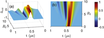
Figure 3. The normalized amplitude of the output pulse  vary with the parameter R2 and time t, when the atom is initially in state
  . Figure (b) is the planform of figure (a). Here we take the parameters
  μs,
μs,  μs and
  .
.
Download figure:
Standard image High-resolution imageNow we focus on the other case, in which an atom is in state  initially. By applying the same procedure as before, one can also find that
  and
and  are always zero. Dynamics of the total system can be described with equations (16), (19), (20) and (28)–(31). In this situation, both the interactions between the atom and reservoir 1, and intracavity-external fields coupling should be taken into account. Similarly, we define parameter
  to characterize the interactions between an atom and reservoir 1. As the atom interacts with reservoir 1 and also with the cavity mode, the corresponding coupling strength are set as
  and
and  , respectively, in figures 4 and 5. We first investigate how the non-Markovian reservoir 1 influences a quantum controlled-PHASE gate. When
  ,
,  μs, the output
  and populations
  under different R1 are shown in figures 4(a) and (b). The non-Markovian numerical results are almost same as the corresponding Markovian limit, even when R1 is as large as 10. For a stronger coupling strength κ, a shorter input optical pulse can be considered, as illustrated in figures 4(c) and (d). The non-Markovian numerical results are in good agreement with those in Markovian approximation when
  . As R1 increases to 10, the memory effects of the non-Markovian environment appear apparently in this short input pulse case. Because the characteristic time scales become comparable with the correlation time of reservoir 1. The excitations which have been leaked into the reservoir 1 can flow back into the atom-cavity system. By the coupling between the single cavity mode and output fields, this memory effect can finally result in a much larger reflectivity, even when the atom-cavity system is in the weak coupling regime. It is quite good for high-speed quantum computation and communication. As we may acquire a short output pulse with 100% reflectivity and π phase-shift, through manipulating parameter
  appropriately, when the atom-cavity coupling is weak. This typical non-Markovian feature would never appear in a Markovian case. For the mutual information exchange between the atom and reservoir 1, more excitations are provided by the cavity field. Thus, as R1 increases, the population
  decreases while
  increases in figure 4(d). Now we take into account the non-Markovian effects caused by the coupling between intracavity and external fields. The parameters in figure 5 are set as same as figure 4, except that we choose
  this time. A larger R2 leads to a longer memory time of the external field, which enhances the back-flowing effects. Hence, the reflectivity increases and populations
  decreases, as shown in figure 5.

Figure 4. Comparison of the normalized output pulses  in non-Markovian approximation for R1 equals 0.1(dotted green line), 10(dashed–dotted magenta line) with the corresponding Markovian limit (dashed–dotted–dotted blue line) are shown in figures (a) and (c), when the atom is initially in state
  . The normalized input Gaussian pulses(solid red line) are also shown here. The numerical results of
  for R1 equals 0.1(dashed red line), 10(dotted green line), and
  for R1 equals 0.1(dashed–dotted–dotted cyan line), 10(short-dashed magenta line) are presented in figures (b) and (d). The corresponding Markovian limit for
  (solid black line) and
  (dashed–dotted blue line) are also illustrated here. Here we take the parameters
  μs,
μs,  μs,
μs,  ,
,  ,
,  in figures (a) and (b),
  μs,
μs,  μs,
μs,  ,
,  ,
,  in figures (c) and (d).
Download figure:
Standard image High-resolution image
Figure 5. Normalized output pulses  calculated in non-Markovian approximation for R2 equals 1(dashed blue line), 10(dashed–dotted magenta line) are shown in figures (a) and (c), when the atom is initially in state
  . The normalized input Gaussian pulses(solid red line) are also shown here. The numerical results of
  for R2 equals 1(solid black line), 10(dotted green line), and
  for R2 equals 1(dashed red line), 10(dashed–dotted blue line) are presented in figures (b) and (d). Here we take the parameters
  μs,
μs,  μs,
μs,  ,
,  ,
,  ,
,  in figures (a) and (b),
  μs,
μs,  μs,
μs,  ,
,  ,
,  ,
,  in figures (c) and (d).
Download figure:
Standard image High-resolution imageFrom the above, it is possible to achieve a deterministic fast controlled-PHASE gate by modulating the reservoirs with the Lorentz type spectral density. When one incidents a short input pulse, the corresponding coupling strength between the cavity and environment should be large. By appropriately increasing R1(decreasing  ) and decreasing R2(increasing
  ), we can implement an ideal deterministic controlled-PHASE gate, even the atom-cavity coupling is weak. As demonstration, for a shorter input pulse with duration time
  μs, the numerical results are illustrated in figure 6, under the parameters
  ,
,  ,
,  and
and  . The simulation results of the corresponding Markovian limits are also shown here as comparison.

Figure 6. Comparison of the normalized output pulses and populations in non-Markovian approximation for  , with the corresponding Markovian limit. Figure (a) shows
  calculated in Markovian(dashed–dotted blue line) or non-Markovian(dashed magenta line) approximation, when the atom is initially in state
  . The population
  in Markovian(solid black line) or non-Markovian(dotted green line) approximation, and
  in Markovian(dashed red line) or non-Markovian(dashed–dotted blue line) approximation are shown in figure (b). Figure (c) shows the
  in non-Markovian approximation(dashed magenta line) and its corresponding Markovian limit(dashed–dotted blue line), when the atom is in state
  . The population
  in Markovian approximation(solid black line) or non-Markovian approximation(dashed blue line) are shown in figure (d). The normalized input Gaussian pulses(solid red line) are shown in figures (a) and (c). Here we take the parameters
  μs,
μs,  μs,
μs,  ,
,  ,
,  .
.
Download figure:
Standard image High-resolution image3.2. Sub-Ohmic, Ohmic and super-Ohmic reservoirs
In this part, we turn to the case in which the two reservoirs have following spectral densities


where  represents the dimensionless coupling strength between
  transition and reservoir 1, and
  is the corresponding cutoff frequency of the spectrum. Similarly, the interaction between the single cavity mode and external field is described by the dimensionless coupling constant
  and cutoff frequency
  . The environment can be classified by the parameter s as sub-Ohmic
  , Ohmic
  and super-Ohmic
  . By applying the same procedure as before, we substitute
 ![$\kappa ({\omega }_{2})={\left[2\pi {\eta }_{2}{\omega }_{2}{\left(\tfrac{{\omega }_{2}}{{\omega }_{c2}}\right)}^{s-1}{{\rm{e}}}^{-\tfrac{{\omega }_{2}}{{\omega }_{c2}}}\right]}^{1/2}$](https://content.cld.iop.org/journals/1367-2630/19/12/123001/revision2/njpaa9510ieqn204.gif) into equation (17) and achieve the response function
into equation (17) and achieve the response function

After substituting equations (34)–(36) into equations (22)–(24), respectively, we can get the following time correlation functions


In the following, we simulate the quantum controlled-PHASE gate by setting the parameter s to 0.1, 1 and 2, respectively. Specifically, we take the single cavity mode frequency  as the norm unit [28]. As stated before, the
  transition is resonantly coupled with the cavity mode, hence
  . The frequency of
  transition is taken as
  . In our numerical calculations, we may roughly set the cutoff frequency
  and
and  , respectively. It should be noted that the Markov limits (equation (32)) are the same for these three spectral densities (
 or 2). Because the parameters
  and
and  are independent of s in this situation. Considering the decay rates of atomic levels, we set
  and
and  , which is corresponding to
  [4]. As the coupling between an atom and reservoir 1 is quite weak, we only simulate the quantum controlled-PHASE gate under different
  ,
,  or
or  (equation (33)). The detailed numerical results are shown in figure 7 through 9.

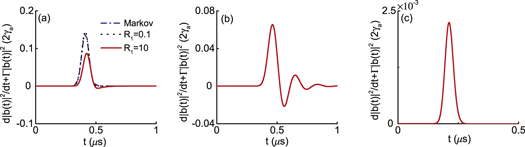
Figure 7. Comparison of the output pulse for sub-Ohmic, Ohmic and super-Ohmic with the corresponding Markovian limit. For figures (a)–(d), the atom is initially in state  , for figures (e)–(h), the atom is initially in state
  . The result in Markovian approximation
  [
[ ] (dashed blue line) is shown in figures (a), (e). The results in non-Markovian approximation, Real[
 ] (Real[
 ])(dotted magenta line), Im[
 ] (Im[
 ])(dashed–dotted black line), and
  [
[ ] (dashed blue line) for sub-Ohmic, Ohmic and super-Ohmic are shown in figures (b), (f), (c), (g) and (d), (h) respectively. The input Gaussian pulse
  [
[ ] (solid red line) is also shown here. Here we take the parameters
  .
.
Download figure:
Standard image High-resolution imageIn figure 7, we show the exact results of output  and
and  when the parameters
  and
and  . An ideal deterministic quantum controlled-PHASE gate can be achieved in the Markovian approximation, which is plotted in figures 7(a) and (e). However, in the non-Markovian case, the influences caused by the memory effects of structured environments become visible, when an atom is initially in state
  . The envelope shape of output pulse is therefore different from the input Gaussian pulse, as shown in figures 7(b)–(d). Moreover, the output
  have both real and imaginary parts, which implies the output light has a time-varied phase-shift changing from
  to π. Although we can achieve the same results as its Markovian limit, when the coupling strength g is large and the atom is initially in state
  , as shown in figures 7(f)–(h). The deterministic quantum controlled-PHASE gates can not be implemented in this situation.
The detailed numerical results with a weaker coupling strength  and a longer input pulse
  are illustrated in figures 8. The parameters are chosen as
  and
and  . When an atom is initially in state
  , the output pulse has exactly the same Gaussian shape as input, which is shown in figures 8(b)–(d). But it still has time-varied phase-shift. When the atom is initially in state
  , one can also get the same output as that in Markovian limit, see figures 8(f)–(h). We furthermore decrease the coupling strength
  to 0.004 and apply a longer input optical pulse
  , the corresponding simulation results are plotted in figure 9. The characters of the output resemble those shown in figure 8.

Figure 8. Comparison of the output pulse for sub-Ohmic, Ohmic and super-Ohmic with the corresponding Markovian limit. For figures (a)–(d), the atom is initially in state  , for figures (e)–(h), the atom is initially in state
  . The result in Markovian approximation
  [
[ ] (dashed blue line) is shown in figures (a), (e). The results in non-Markovian approximation, Real[
 ] (Real[
 ])(dotted magenta line), Im[
 ] (Im[
 ])(dashed–dotted black line), and
  [
[ ] (dashed blue line) for sub-Ohmic, Ohmic and super-Ohmic are shown in figures (b), (f), (c), (g) and (d), (h) respectively. The input Gaussian pulse
  [
[ ] (solid red line) is also shown here. Here we take the parameters
  .
.
Download figure:
Standard image High-resolution image
Figure 9. Comparison of the output pulse for sub-Ohmic, Ohmic and super-Ohmic with the corresponding Markovian limit. For figures (a)–(d), the atom is initially in state  , for figures (e)–(h), the atom is initially in state
  . The result in Markovian approximation
  [
[ ] (dashed blue line) is shown in figures (a), (e). The results in non-Markovian approximation, Real[
 ] (Real[
 ])(dotted magenta line), Im[
 ] (Im[
 ])(dashed–dotted black line), and
  [
[ ] (dashed blue line) for sub-Ohmic, Ohmic and super-Ohmic are shown in figures (b), (f), (c), (g) and (d), (h) respectively. The input Gaussian pulse
  [
[ ] (solid red line) is also shown here. Here we take the parameters
  .
.
Download figure:
Standard image High-resolution imageIn our chosen parameters, in the weak coupling regime( ), the exact envelope shape of output pulse
  [
[![$| {\tilde{a}}_{\mathrm{out}}(t)| ]$](https://content.cld.iop.org/journals/1367-2630/19/12/123001/revision2/njpaa9510ieqn278.gif) is almost same as the corresponding Markovian limit, i.e. as same as the shape of the input pulse
is almost same as the corresponding Markovian limit, i.e. as same as the shape of the input pulse  [
[ ]. Though a π phase shift can be acquired as an atom initially in state
  , the phase shift of the output pulse is time-varied with the atom at state
  . Such phase shift in the output pulse hinders the implementation of an ideal deterministic controlled-PHASE gate in sub-Ohmic, Ohmic or super-Ohmic environments.
3.3. Insight into the physical mechanism
We have seen that the deterministic quantum controlled-PHASE gates can only be realized in the Lorentzian reservoirs. The key point in this realization is that the memory effects of the Lorentzian reservoir 1 can be utilized, especially when the atom-cavity coupling is weak, as shown in figures 4(c) and 6(a). To confirm the results above, here we present some insights into the physical mechanism, by making use of the pseudomode theory [42–44]. In the pseudomode method, the pseudomodes are defined by the positions and residues of the poles of the reservoir spectrum [42]. The dynamics of a system interacting with a structured reservoir can be equivalently described by the coherent coupling between the system and pseudomodes, and the latter one leaking into an independent Markovian reservoir [42].
When the reservoir 1 has a Lorentzian spectrum, equation (20) can be rewritten as

where  and
and  represent the amplitudes of the two pseudomodes, respectively.


The oscillation frequencies of these two pseudomodes are  and
and  , the decay rates are
  and
and  , respectively, which are defined by the poles of reservoir spectrums equations (25) and (26).
  and
and  denote the coupling strengths between the atom and two pseudomodes, respectively. A smaller
  (
( ) implies a weaker coupling strength
  (
( ). As previously, we assume
  ,
,  (
( ). We can get the total population of the two pseudomodes

In our article, the atom is not only coupled with these two pseudomodes, but also interacts with the single cavity mode. After considering the effects of the pseudomodes leakage, one can directly analyze the energy flowing between the atom and reservoir 1, from the compensated rate of change of the total pseudomode population  [44].
[44].
When R1 equals 0.1, the compensated rate of change  is almost as same as the decay rate of the excited state population of the atom in Markovian limit
  , as illustrated in figure 10(a). A larger R1(smaller
  ) results in a weaker coupling strength
  (or
(or  ) between the atom and pseudomodes, while the atom-cavity coupling is strong. In this condition, more excitations tend to transfer between the atom and single cavity mode, while less excitations are exchanged between the atom and pseudomodes, as shown in figure 10. When R1 gets much larger, the atom is almost decoupled from the pseudomodes, and almost none excitations transfer to the pseudomodes, as depicted in figure 10(c), which brings about the excellent results in figure 6(a). This phenomenon can be viewed as the net effects due to the backflowing of the environments. Actually, the changes of parameter R1 only affect the memory time(
 ) of reservoir 1, and the coupling strength γ between the atom and reservoir 1 is unchanged. It should be noted that the compensated rate of change has some negative values, which implies the population of the pseudomodes transfer back to the atom. It is a consequence of the memory effects of environments. As the atom-cavity coupling strength gets much weaker, the interaction between the atom and pseudomodes plays a more important role, the compensated rate of change oscillates in a more intuitive way in this time, as shown in figure 10(b).
Figure 10. Comparison of the compensated rate of change of the total pseudomode population  in non-Markovian approximation for R1 equals 0.1(dotted black line), 10(solid red line) with the corresponding Markovian limit
  (dashed–dotted blue line) is shown in figure (a), the atom-cavity coupling strength g is
  . The results in figure (a) are corresponding to figures 4(c) and (d). Figure (b) shows the compensated rate of change
  for R1 equals 10, when the atom-cavity coupling strength g is
  . In figures (a) and (b), we take the parameters
  μs,
μs,  μs,
μs,  ,
,  ,
,  . Figure (c) shows the compensated rate of change
  for R1 equals 150. The result in figure (c) is corresponding to figures 6(a) and (b). Here we take the parameters
  μs,
μs,  μs,
μs,  ,
,  ,
,  ,
,  . The units for the rates on the vertical axes are
  .
.
Download figure:
Standard image High-resolution image
For a reservoir with a Lorentzian spectrum, one can utilize the above pseudomode theory to interpret the physics. However, this pseudomode method can not be used for sub-Ohmic, Ohmic or super-Ohmic reservoirs, as there exists no such poles in these reservoir spectrums. In our study of sub-Ohmic, Ohmic or super-Ohmic reservoirs, the phase shift of the output pulse is time-varied with the atom at state  .
.
4. Discussion
As we stated before, the deterministic quantum controlled-PHASE gate can only be constructed in a Lorentzian reservoir, but not a sub-Ohmic, Ohmic or super-Ohmic reservoir. One can identify the Lorentzian reservoir and Ohmic reservoir by making use of the methods of noise spectroscopy. Many experimental and theoretical studies have been focused on measuring the noise spectrums [45–49]. For example, by utilizing the dynamical decoupling, we can recognize an unknown noise spectrum, after applying appropriate pulse sequences and measuring the decay rates [45, 46, 48, 49]. Given that there exists the connection between the noise spectrums and some observables, one can also identify the noise spectrums by measuring the expectation values of observables [47]. These methods stated above can be used for reference in our system to identify noise.
In many experimental architectures, due to inevitable effect from the surrounding environment, the real system cannot be seen as a closed system, and the noise should be taken into consideration. The existence of the systems with Lorentz spectrums has been demonstrated in many situations. An atom placed inside a lossy cavity is a typical example of a system interacting with such engineered structured reservoirs [43, 44, 50]. The electromagnetic field inside a lossy cavity can be viewed as a reservoir with Lorentzian spectrum. By manipulating the parameters of a cavity, one can control the parameters of the Lorentzian reservoir spectrum. Our study can also be applied to many other systems, e.g., a superconducting artificial atom coupled to a superconducting transmission-line resonator (TLR) [14, 51]. TLRs can be viewed as microwave cavities, which can filter the input white noise into the non-Markovian noise with Lorentzian spectrums [51].
5. Conclusion
In conclusion, we theoretically studied the construction of a quantum controlled-PHASE gate between a single photon and an atom coupled to a single-sided cavity. Here, we derive the dynamics of the atom-cavity system under general conditions, and the memory backflow from the non-Markovian reservoir is counted. Both the coupling between an atom and the reservoir, and the interaction between the cavity mode and the environment have been taken into account. We numerically calculated the output field of the controlled-PHASE gate under different parameters, in various structured environments. We found that, when spectral density of the reservoir is the Lorentz type, whatever the coupling strength between the atom and cavity is strong or weak, it is possible to implement an ideal deterministic controlled-PHASE gate by appropriately manipulating the system parameters, which can not happen in study with the Markovian approximation. This feature induced by the back-flowing phenomenon can benefit the rapid quantum communication and computation. Moreover, we also investigated the performance of a quantum controlled-PHASE gate in environments with sub-Ohmic, Ohmic, and super-Ohmic spectrums. We found that, the phase shift in the output pulse hinders the implementation of quantum controlled-PHASE gates in these reservoirs.
Acknowledgments
We acknowledge support from Shandong Province, the National High-Tech Program of China Grants No. 2011AA010801 and No. 2011AA010803, and NSFC Grants No. 11174177, No. 11474182 and No. 60725416.