


Abstract
We consider active particles swimming in a convergent fluid flow in a trapezoid nozzle with no-slip walls. We use mathematical modeling to analyze trajectories of these particles inside the nozzle. By extensive Monte Carlo simulations, we show that trajectories are strongly affected by the background fluid flow and geometry of the nozzle leading to wall accumulation and upstream motion (rheotaxis). In particular, we describe the non-trivial focusing of active rods depending on physical and geometrical parameters. It is also established that the convergent component of the background flow leads to stability of both downstream and upstream swimming at the centerline. The stability of downstream swimming enhances focusing, and the stability of upstream swimming enables rheotaxis in the bulk.
Export citation and abstract BibTeX RIS
1. Introduction
Active matter consists of a large number of self-driven agents converting chemical energy, usually stored in the surrounding environment, into mechanical motion [1–3]. In the last decade various realizations of active matter have been studied including living self-propelled particles as well as synthetically manufactured ones. Living agents are for example bacteria [4, 5], microtubules in biological cells [6, 7], spermatozoa [8–10] and animals [11–13].
Such systems are out-of-equilibrium and show a variety of collective effects, from clustering [14–17] to swarming, swirling and turbulent type motions [3–5, 13, 18–21], reduction of effective viscosity [22–28], extraction of useful energy [29–31], and enhanced mixing [32–34]. Besides the behavior of microswimmers in the bulk the influence of confinement has been studied intensively in experiments [35, 36] and numerical simulations [37–41]. There are two distinguishing features of swimmers confined by walls and exposed to an external flow: accumulation at the walls and upstream motion (rheotaxis). Microorganisms such as bacteria [42–46] and sperm cells [47] are typically attracted by no-slip surfaces. Such accumulation was also observed for larger organisms such as worms [48] and for synthetic particles [49]. The propensity of active particles to turn themselves against the flow (rheotaxis) is also typically observed. While for larger organisms, such as fish, rheotaxis is caused by a deliberate response to a stream to hold their position [50], for micron sized swimmers rheotaxis has a pure mechanical origin [51–55].
These phenomena observed in living active matter can also be achieved using synthetic swimmers, such as self-thermophoretic [56] and self-diffusiophoretic [57–60] micron sized particles as well as particles set into active motion due to the influence of an external field [61–63].
Using simple models we describe the extrusion of a dilute active suspension through a trapezoid nozzle. We analyze the qualitative behavior of trajectories of an individual active particle in the nozzle and study the statistical properties of the particles in the nozzle. The accumulation at walls and rheotaxis are important for understanding how an active suspension is extruded through a nozzle. Wall accumulation may eliminate all possible benefits caused by the activity of the particles in the bulk. Due to rheotaxis active particles may never reach the outlet and leave the nozzle through the inlet, so that properties of the suspension coming out through the outlet will not differ from those of the background fluid.
The specific geometry of the nozzle is also important for our study. The nozzle is a finite domain with two open ends (the inlet and the outlet) and the walls of the nozzle are not parallel but convergent, that is, the distance between walls decreases from the inlet to the outlet. The statistical properties of active suspension (e.g., concentration of active particles) extruded in the infinite channel with parallel straight or periodic walls are well-established, see e.g., [64] and [65], respectively. The finite nozzle size leads to a 'proximity effect', i.e., the equilibrium distribution of active particles changes significantly in proximity of both the inlet and the outlet. The fact that the walls are convergent, results in a 'focusing effect', i.e., the background flow compared to the pressure driven flow in the straight channel (the Poiseuille flow) has an additional convergent component that turns a particle toward the centerline. Specifically, in this work it is shown that due to this convergent component of the background flow both up- and downstream swimming at the centerline are stable. Stability of the upstream swimming at the centerline is somewhat surprising since from observations in the Poisueille flow it is expected that an active particle turns against the flow only while swimming towards the walls, where the shear rate is higher. This means that we find rheotaxis in the bulk of an active suspension.
2. Model
To study the dynamics of active particles in a converging flow, two modeling approaches are exploited. In both, an active particle is represented by a rigid rod of length ℓswimming in the xy-plane. In the first—simpler—approach, the rod is a one-dimensional segment which cannot penetrate a wall, whereas in the second—more sophisticated—approach we use the Yukawa segment model [66] to take into account both finite length and width of the rod, as well as a more accurate description of particle–wall steric interaction.
The active particle's center location and its unit orientation vector are denoted by  and
and  , respectively. The active particles are self-propelled with a velocity directed along their orientation
  . The active particles are confined by a nozzle, see figure 1, which is an isosceles trapezoid Ω, placed in the xy-plane so that inlet
  and outlet
  are bases and the y-axis is the line of symmetry:

The nozzle length, the distance between the inlet and the outlet, is denoted by L, i.e.,  . The width of the outlet and the inlet are denoted by
  and
and  , respectively, and their ratio is denoted by
  .
.
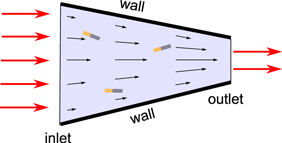
Figure 1. Sketch of a trapezoid nozzle filled with a dilute suspension of rod-like active particles in the presence of a converging background flow illustrated by black arrows.
Download figure:
Standard image High-resolution imageFurthermore, the active particles are exposed to an external background flow. We approximate the resulting converging background flow due to the trapezoid geometry of the nozzle by

where u0 is a constant coefficient related to the flow rate and α is the slope of walls of the nozzle (see also the appendix). Equation (2) is an approximation of the Poiseuille flow to channels with convergent walls5 .
Active particles swim in the low Reynolds-number regime. The corresponding overdamped equations of motion for the locations  and orientations
  are given by:


Here (4) is the Jeffery's equation [20, 67, 68] for rods with an additional term due to random reorientation with rotational diffusion coefficient Dr; ζ is an uncorrelated noise with the intensity  ,
,  . Equation (4) can also be rewritten for the orientation angle φ:

The torque exerted by the background flow  on active particles is described by
  ,
,  , and
, and  the local vorticity, vertical expansion (or, equivalently, horizontal compression; similar to Poisson's effect in elasticity) and shear. In the first approach, the torque is calculated for point-like representation of the particle.
The strength of the background flow is quantified by the inverse Stokes number, which is the ratio between the background flow at the center of the inlet and the self-propulsion velocity v0. Specifically,

where  denotes the location at the center of the inlet.
In the first modeling approach we mimic particle–wall interactions by hard core collisions in the following way: an active particle is not allowed to penetrate the walls of the nozzle. To enforce this, we require that both the front and the back of the particle,  , are located inside the nozzle. In numerical simulations of the system (3)–(5), this requirement translates into the following rule: if during numerical integration of (3)–(5) a particle penetrates one of the two walls, then this particle is instantaneously shifted back along the inward normal at the minimal distance, so its front and back are again located inside the nozzle while its orientation is kept fixed to avoid a specifically chosen alignment rule.
Unless mentioned otherwise, in this modeling approach we consider a nozzle whose inlet width  and outlet width
  are fixed. The following nozzle lengths are considered:
  ,
,  and
and  . The length of the active particles is
  μm, they swim with a self-propulsion velocity
  μm
μm  and their rotational diffusion coefficient is given by Dr = 0.1
  .
.
All active particles are initially placed at the inlet,  , with random y-component y(0) and orientation angle
  . The probability distribution function for initial conditions y(0) and
  is given by
  (uniform). The trajectory of an active particle is studied until it leaves the nozzle either through the inlet or the outlet. To gather statistics we use 96 000 trajectories.
We use the second approach to describe the particle–wall interactions and the torque induced by the flow more accurately. For this purpose each rod, representing an active particle, of length ℓ, width λ and the corresponding aspect ratio  is discretized into nr spherical segments with
  (
( denotes the nearest integer function). The segments are placed along the backbone of each particle to create a stiff rod-like particle. The resulting segment distance is also used to discretize the walls of the nozzle into nw segments in the same way. Between the segments of different objects a repulsive Yukawa potential is imposed. The resulting total pair potential is given by
 ![$U={U}_{0}{\sum }_{i=1}^{{n}_{r}}{\sum }_{j=1}^{{n}_{{\rm{w}}}}\exp [-{r}_{{ij}}/\lambda ]/{r}_{{ij}}$](https://content.cld.iop.org/journals/1367-2630/19/11/115005/revision2/njpaa94fdieqn44.gif) , where λ is the screening length defining the particle diameter, U0 is the prefactor of the Yukawa potential and
, where λ is the screening length defining the particle diameter, U0 is the prefactor of the Yukawa potential and  is the distance between segment i of a rod and j of the wall of the nozzle, see figure 2.
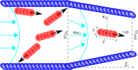
Figure 2. Sketch of a discretized active rod (red) of length ℓand width λ which is propelled with a velocity v0 along its orientation  and is exposed to a converging background flow
  in the presence of a trapezoid nozzle confinement of length L and with an inlet of size
  and outlet of size
  (blue). To study a system with a packing fraction
  , a channel is attached to the inlet with a non-converging background flow.
Download figure:
Standard image High-resolution imageThe equations of motion (3) and (4) are complemented by the respective derivative of the total potential energy of a rod along with the one-body translational and rotational friction tensors for the rods  and
and  which can be decomposed into parallel
  , perpendicular
  and rotational
  contributions which depend solely on the aspect ratio a [69]. In this second approach, the torque exerted by the flow on the particles contains two components. The first one is the torque acting on its center of mass, as in the previous approach (see again equation (5)). The second one is the torque due to forces acting on the extended body. Note that we neglect any further hydrodynamic interactions in this model and so the active particles do not alter the flow. For this approach we measure distances in units of λ, velocities in units of
  (here F0 is an effective self-propulsion force), and time in units of
  . While the width of the outlet
  is varied, the width of the inlet
  as well as the length of the nozzle L is fixed to
  in our second approach. Initial conditions are the same as in the first approach. To avoid that a rod and a wall initially intersect each other, the rod is allowed to reorient itself during an equilibration time
  while its center of mass is fixed.
Furthermore, we use the second approach to study the impact of a finite density of swimmers. For this approach we initialize N active rods in a channel confinement which is connected to the inlet of the nozzle, see figure 2. Inside the channel we assume a regular (non-converging) Poiseuille flow [70]. We restrict our study to a dilute active suspension with a two dimensional packing fraction  . To maintain this fraction, particles which leave the simulation domain are randomly placed at the inlet of the channel confinement.
3. Results
3.1. Focusing of outlet distribution
Here we characterize the properties of the particles leaving the nozzle at either the outlet or the inlet. Specifically, our objective is to determine whether particles accumulate at the center or at walls when they pass through the outlet or the inlet.
We start with the first modeling approach. Figure 3 shows the spatial distribution of active particles leaving the nozzle at the outlet for various inverse Stokes number σ and three different lengths L of the nozzle, while the width of the inlet and the outlet are fixed. For small inverse Stokes number σ, the background flow is negligible compared to the self-propulsion velocity. Active particles swim close to the walls and peaks at walls are still clearly visible for  for all nozzle lengths L, see figure 3(a). For
  , the self-propulsion velocity and the background flow are comparable; in this case the histogram shows a single peak at the center of the outlet, see figure 3(b). Further increasing the inverse Stokes number from
  to
to  leads to a broadening of the central peak and then to the formation of two peaks with a well in the center of the outlet, see figures 3(c)–(e). Finally, for an even larger inverse Stokes number σ, the self-propulsion velocity is negligible and the histogram becomes close to the one in the passive (no self-propulsion,
  ) case, see figure 3(f). Here the histogram for a nozzle length
  is uniform except at the edges where it has local peaks due to accumulation at the walls caused by steric interactions.
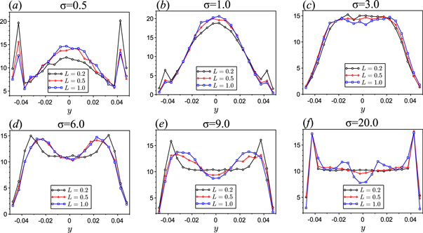
Figure 3. Histograms of the outlet distribution for  for given inverse Stokes number σ and length L of the nozzle. The histograms are obtained from numerical integration of (3)–(5).
Download figure:
Standard image High-resolution imageHistograms for both the y-component and the orientation angle φ of the active particles reaching the outlet are depicted in figures 4(a)–(c). While active particles leave the nozzle with orientations away from the centerline for small inverse Stokes number,  , they are mostly oriented towards the centerline for larger values of the inverse Stokes number. In figure 4(c), one can observe that the histogram is concentrated largely for downstream orientations
  and slightly for upstream orientations
  . These local peaks for
  away from walls are evidence of rheotaxis in the bulk. These peaks are visible for large inverse Stokes numbers only and the corresponding active particles are flushed out of the nozzle with upstream orientations.

Figure 4. Outlet distribution histograms for  computed for given inverse Stokes number σ and nozzle length L = 0.2.
Download figure:
Standard image High-resolution imageDue to rotational diffusion and rheotaxis it is possible that an active particle can leave the nozzle through the inlet. We compute the probability of active particles to reach the outlet. This probability, as a function of the inverse Stokes number σ for the three considered nozzle lengths L, is shown in figure 5(a), together with selected trajectories, see insets in figure 5(a). The figure shows that the probability that an active particle eventually reaches the outlet monotonically grows with the inverse Stokes number σ. Note that a passive particle always leaves the nozzle through the outlet. By comparing the probabilities for different nozzle lengths L it becomes obvious that an active particle is less likely to leave the nozzle through the outlet for longer nozzles. Due to the larger distance L between the inlet and the outlet an active particle spends more time within the nozzle, which makes it more likely to swim upstream by either rotational diffusion or rheotaxis. In figures 5(b)–(d) histograms for active particles leaving the nozzle through the inlet are shown. In the case of small inverse Stokes number,  , the majority of active particles leaves the nozzle at the inlet. Specifically, most of them swim upstream due to rheotaxis close to the walls, but some active particles leave the nozzle at the inlet close to the center. These active particles are oriented upstream due to random reorientation. By increasing the inverse Stokes number
  , active particles are no longer able to leave the nozzle at the inlet close to the center.

Figure 5. (a) Probability of active particles to reach the outlet for various inverse Stokes number σ (horizontal axis) and given lengths of the nozzle L. Insets: trajectories for the case of  . (b)–(d) Distribution histograms for particles leaving the nozzle through the inlet
  computed for given reduced flow velocities σ and nozzle lengths L.
Download figure:
Standard image High-resolution imageLet us now consider specific examples of active particles' trajectories, see figure 6. The first trajectory (red) starts and ends at the inlet. Initially the active particle swims downstream and collides with the upper wall due to the torque induced by the background flow. Close to the wall it exhibits rheotactic behavior, but before it reaches the inlet it is expelled towards the center of the nozzle due to rotational diffusion, similar to bacteria that may escape from surfaces due to tumbling [71] or other swimmers due to rotational diffusion [35, 72]. Eventually, the active particle leaves the nozzle at the inlet. As for the other depicted trajectory (blue), the active particle manages to reach the outlet. Along its course through the nozzle it swims upstream several times but in the end the active particle is washed out through the outlet by the background flow. For larger flow rates the trajectories of active particles are less curly, since the flow gets more dominant, see insets of figure 5(a). In both representations we can observe the guidance of active particles along the channel wall. The swimmers tend to zigzag and bounce off opposite walls, especially in a narrow confinement [37, 40, 73–75].
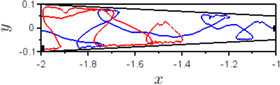
Figure 6. Examples of two trajectories for L = 1 mm and  . The red trajectory starts and ends at the inlet (the endpoint is near the lower wall). The blue trajectory has a zigzag shape with loops close to the walls; the particle that corresponds to the blue trajectory manages to reach the outlet. Supplementary videos show how a particle exhibits the trajectories depicted in this figure.
Download figure:
Standard image High-resolution imageNext we present results of the second modeling approach which is based on the Yukawa segment model. So far we have concentrated on fixed widths of the inlet and outlet. Here we consider nozzles with fixed length L and inlet width  and vary nozzle ratio k. We study the behavior of active rods with varied aspect ratio a. In agreement with the first model, the probability
  , which measures how many active rods leave the nozzle at the outlet, increases with increasing inverse Stokes number σ. But as shown in figure 7, neither the aspect ratio a, see figure 7(a), nor the nozzle ratio k, see figure 7(b), have a significant impact on the probability
  . However, the aspect ratio a is important for the location where the active rods leave the nozzle at the inlet and the outlet, see figure 8. For short rods
  and small inverse Stokes numbers
  the distribution of active particles shows just a single peak located at the center. This peak at the centerline broadens if the inverse Stokes number increases, which is in perfect agreement with the results obtained by the first approach, see figure 3. It is more likely for short rods than for long ones to be expelled towards the center due to rotational diffusion. Hence the distribution of particles at the outlet for long rods
  shows additional peaks close to the wall. These peaks become smaller if the inverse Stokes number increases. The distribution of particles leaving the nozzle at the inlet is similar to our first approach. While the distribution is almost flat for small inverse Stokes numbers, increasing this number makes it impossible to leave the nozzle close to the center at the inlet. Similar to the outlet the wall accumulation at the inlet is more pronounced for longer rods.

Figure 7. (a) Probability for an active particle to reach the outlet of the nozzle  as a function of inverse Stokes number σ for three given aspect ratios a of self-propelled rods and (b) for a fixed aspect ratio a and three given ratios of the nozzle k. Insets show close-ups.
Download figure:
Standard image High-resolution image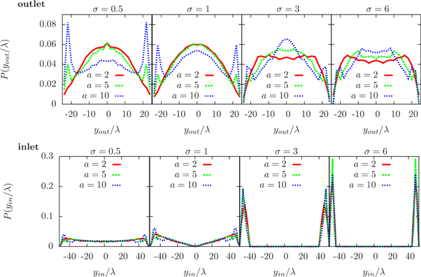
Figure 8. Comparison of the spatial distribution of active particles at (top row) the outlet and (bottom row) the inlet of the nozzle for given inverse Stokes numbers σ and aspect ratios a, an outlet width  and an inlet width
  .
.
Download figure:
Standard image High-resolution imageBy comparing the orientation of the particles at the outlet, the influence of the actual length of the rod becomes visible, see figure 9. As seen before for short rods, a = 2, for small inverse Stokes numbers σ there is no wall accumulation. Hence most particles leave the nozzle close to the center and are oriented in the direction of the outlet. This profile smears out if the inverse Stokes number is increased to  . For larger inverse Stokes numbers the figures are qualitatively similar to the one obtained by the first approach, see figure 4(c). Particles in the bottom half of the nozzle tend to point upwards and particles in the top half tend to point downwards. The same tendency is seen for long rods a = 10 with small inverse Stokes number. However for long active rods, this is because they slide along the walls. The bright spots close to the walls in figure 9 for long rods and large inverse Stokes numbers indicate that particles close to the walls are flushed through the outlet by the large background flow even if they are oriented upstream. In addition, there are blurred peaks away from the walls for large inverse Stokes numbers σ. The corresponding particles cross the outlet with mostly upstream orientations. This is similar to figure 4(c), where particles exhibiting in-bulk rheotactic characteristics were observed at the outlet of the nozzle.
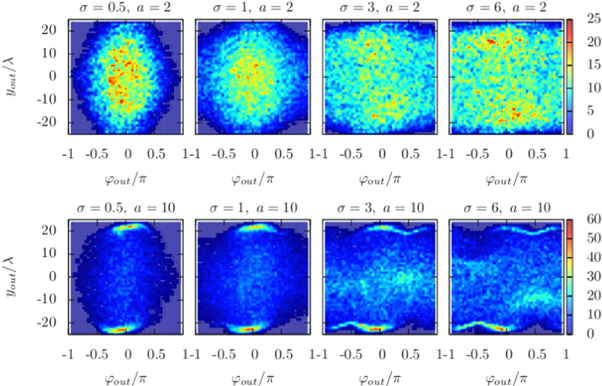
Figure 9. Outlet distribution histograms for  computed for given inverse Stokes numbers σ and a nozzle with an outlet width of
  for active rods with an aspect ratio (top row) a = 2 and (bottom row) a = 10.
Download figure:
Standard image High-resolution imageBy comparing the results for individual active rods, see again figure 9, with those for interacting active rods at a finite packing fraction  , see figure 10, we find that wall accumulation becomes more pronounced. Mutual collisions of the rods lead to a broader distribution of particles. For long rods, a = 10, the peaks at
  and
and  remain close to the walls and the blurred peaks at the center vanish.
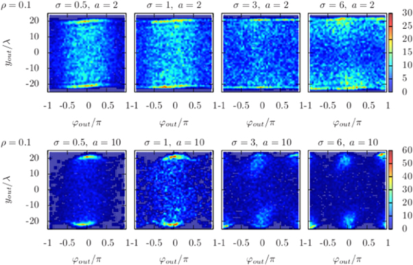
Figure 10. Outlet distribution histograms for  computed for given inverse Stokes numbers σ and a nozzle with an outlet width
  for active rods with an aspect ratio (top row) a = 2 and (bottom row) a = 10 for a packing fraction
  .
.
Download figure:
Standard image High-resolution image3.2. Optimization of focusing
Here we study the properties of the active particles in more detail and provide insight into the nozzle geometry, the background flow and the size of the swimmers that should be used in order to optimize the focusing at the outlet of the nozzle.
For this purpose we study three distinct quantities. The averaged dwell time  , the time it takes for an active particle to reach the outlet, the mean alignment of the particles measured by
  and the mean deviation from the center y = 0 at the outlet
  . As depicted in figure 5, for increasing inverse Stokes number the probability for active particles to reach the outlet increases. However they are spread all over the outlet. This is quantified by the
  . Small values of
  correspond to a better focusing. If particles leave the nozzle with no preferred orientation, their mean orientation vanishes,
  in case of being oriented upstream we obtain
  and finally
  if the particles are pointing in the direction of the outlet. Obviously in an experimental realization a fast focusing process and hence small dwell times T would be preferable.
The numerical results obtained by the first modeling approach are depicted in figure 11. While the dwell time hardly depends on the size ratio k of the nozzle, obviously the strength of the background flow has a strong impact on the dwell time and large inverse Stokes numbers σ lead to a faster passing through the nozzle of the active particles, see figure 11(a). The alignment of active particles,  , becomes better if the nozzle ratio k is large and the flow is slow, see figure 11(b). The averaged deviation from the centerline
  increases with increasing nozzle ratio k since the width of the outlet becomes larger. As could already be seen in figure 3, the averaged deviation from the centerline is non-monotonic as a function of the inverse Stokes number and shows the smallest distance from the centerline for all nozzle ratios if the strength of the flow is comparable to the self-propulsion velocity of the swimmers,
  .
.
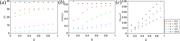
Figure 11. (a) Dwell time  (b) mean alignment at the outlet,
  (c) mean deviation from center y = 0 at the outlet
  .
.
Download figure:
Standard image High-resolution imageLet us now discuss how these three quantities depend on the aspect ratio of the swimmer. To this end, we use the second modeling approach. We consider all three parameters as a function of the inverse Stokes number σ. Longer rods have a shorter dwell time so that they reach the outlet faster, see figure 12(a). Increasing the flow velocity obviously leads to a decreasing dwell time. The same holds for the mean alignment—it decreases for increasing inverse Stokes number, see figure 12(b). Moreover, for small inverse Stokes numbers,  , the mean alignment is better for long rods. For large inverse Stokes numbers, long rods a = 10 are washed out with almost random orientation, however short rods a = 2 are slightly aligned with the flow. Short rods are focused better for small inverse Stokes numbers,
  , see figure 12(c), due to wall alignment and wall accumulation of longer rods. For larger inverse Stokes numbers, it is the other way around—long rods are better focused. Comparing various nozzle ratios k with fixed simmers' aspect ratio a, we obtain that smaller ratios k lead to smaller dwell times (figure 12(d)) and better alignment (figure 12(e)). For narrow outlets (small k) the active particles leave the outlet closer to the center, see figure 12(f).

Figure 12. (a, e) Dwell time  , (b, f) the mean alignment,
  and (c, f) mean deviation from center y = 0 at the outlet
  for (top row) a fixed outlet width of
  and given aspect ratios a of the swimmers and (bottom row) fixed aspect ratio a = 2 and varied nozzle ratio k, whereby the width of the outlet changes.
Download figure:
Standard image High-resolution image4. Discussion
We discuss the stability of particles around the centerline y = 0 in the presence of a background flow and confining walls if they are converging with a non-zero slope α. This stability is in contrast to a channel with parallel walls, where an active particle swims away from the centerline provided that its orientation angle φ is different from  ,
,  .
.
Indeed, in the case of a straight channel,  , the background flow is defined as
  , uy = 0 (Poiseuille flow; u0 is the strength of the flow,
  is the distance between the walls). Then the system (3)–(5) reduces to


Here we omit the equation for x(t) due to invariance of the infinite channel with respect to x and neglect orientation fluctuations, that is Dr = 0. The phase portrait for this system is depicted in figure 13(a). Dashed vertical lines  ,
,  consist of stationary solutions: if an active particle is initially oriented parallel to the walls, it keeps swimming parallel to them. If initially φ is different from
  , then the active particle swims away from the centerline,
  as
as  .
.
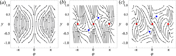
Figure 13. Phase portraits  for v = 0.2, H = 1.0 and u0 = 0.6. (a) System (7) and (8), describing Poiseuille flow in a parallel channel; dashed lines consist of stationary points. (b) System (9) and (10) describing a simplified convergent flow with
  ; stationary points: stable
  (in red) and pairs of saddles with non-zero y (in blue).Trajectories near the centerline converge to a stationary solution in the centerline. (c) System (3)–(5) with the convergent flow
  used in section 3.1 with
  .
.
Download figure:
Standard image High-resolution imageWhen the walls are converging,  , the y-component of the background flow is non-zero and directed towards the centerline. For the sake of simplicity we take
  ,
,  and ux as in the Poiseuille flow,
  . In this case, the system (3)–(5) reduces to


The corresponding phase portrait for this system is depicted in figure 13(b). Orientations  represent stationary solutions only if y = 0. In contrast to the Poiseuille flow in a parallel channel, see equations (7) and (8), these stationary solutions
  are asymptotically stable with a decay rate α (recall that α is the slope of walls). In addition to these stable stationary points there are pairs of unstable (saddle) points with non-zero y (provided that
  ). In these saddle points, the distance from centerline
  does not change, since a particle is oriented away from centerline, so the propulsion force moves the particle away from the centerline and this force is balanced by the convergent component of the background flow, uy, moving the particle toward the centerline. The orientation angle φ does not change since the torque from the Poiseuille component of the background flow, ux, is balanced by the torque from the convergent component, uy.
We also draw the phase portrait for the converging flow  introduced in section 2, figure 13(c). One can compare the phase portraits figures 13(b) and (c) around the stationary point
  to see that the qualitative picture is the same: this stationary point is stable and it neighbors with two saddle points.
The asymptotic stability of  means that if a particle is close to the centerline and its orientation angle is close to 0 (particle is oriented towards the outlet), it will keep swimming at the centerline pointing toward the outlet, whereas in Poiseuille flow the particle would swim away. The asymptotic stability of
  is an evidence of that in the converging flow there is rheotaxis not only at walls but also in the bulk, specifically at the centerline. Another consequence of this stability is the reduction of effective rotational diffusion of an active particle in the region around the centerline, that is the mean square angular displacement
  is bounded in time due to the presence of restoring force coming from the converging component of the background flow (see diffusion quenching for Janus particles in [49]). Finally, we note that the nozzle has a finite length L and thus, the conclusions of the stability analysis are valid if the stability relaxation time,
  s, does not exceed the average dwell time
  . We introduce a lower bound
  for the dwell time
  as the dwell time of an active particle swimming along the centerline oriented forward,
  :
:

Our numerical simulations show that  underestimates the average dwell time by a factor larger than two. Using this lower bound, we obtain the following sufficient condition for stability:
  .
.
5. Conclusion
In this work we study a dilute suspension of active rods in a viscous fluid extruded through a trapezoid nozzle. Using numerical simulations we examined the probability that a particle leaves the nozzle through the outlet—which is the result of the two counteracting phenomena. On the one hand, swimming downstream together with being focused by the converging flow increases the probability that an active rod leaves the nozzle at the outlet. On the other hand, rheotaxis results in a tendency of active rods to swim upstream.
Theoretical approaches introduced in this paper can be used to design experimental setups for the extrusion of active suspensions through a nozzle. The optimal focusing is the result of a compromise. While for large flow rates it is very likely for active rods to leave the nozzle through the outlet very fast, their orientation is rather random and they pass through the outlet close to the walls. The particles are much better aligned with the flow for small flow rates and focused closer to the centerline of the nozzle, however the dwell time of the particles becomes quite large. Based on our findings the focusing is optimal if the velocity of the background flow and the self-propulsion velocity of the active rods are comparable. To reduce wall accumulation, the rods should have a small aspect ratio.
We find that rheotaxis in bulk is possible for simple rigid rod-like active particles. We also established analytically the local stability of active particle trajectories in the vicinity of the centerline. This stability leads to the decrease of the effective rotational diffusion of the active particles in this region as well as the emergence of rheotaxis away from walls. Our findings can be experimentally verified using biological or artificial swimmers in a converging flow [76] and should be extended to study the influence of hydrodynamic interactions.
Acknowledgments
The work of MP and LB was supported by National Science Foundation (DMREF-1628411). The work of ISA was supported by National Science Foundation (DMREF-1735700). AK gratefully acknowledges financial support through a Postdoctoral Research Fellowship (KA 4255/1-2) from the Deutsche Forschungsgemeinschaft (DFG).
Author contributions statement
Simulations have been performed by MP and AK, the research has been conceived by LB and ISA and all authors wrote the manuscript.
Appendix.: On the background flow 

Let us show here the derivation of the background flow  . We search for
  in the following form:

Here f and g are unknown functions of variable x, and m is an arbitrary integer. Let us explain why we chose this ansatz. The presence of the term  in both ux and uy guarantees no-slip boundary conditions, that is the background flow vanishes at walls, and the walls are geometrically described by the equation
  . An even power of y,
  , in ux is chosen so that the flow is symmetric around the centerline y = 0 and it is always co-directed with x-axis. An odd power of y,
  , in uy is because the flow is oriented toward the centerline: uy is negative for
  (above the centerline) and uy is positive for
  (below the centerline).
To find f and g we use incompressibility of the fluid,  :
:

Matching coefficients in front of different powers of y gives  and
and  , where cm is an arbitrary constant.
From the fact that the problem of finding an admissible flow is linear, we write a more general form for  :
:

Or, in the vectorial form, the background flow can be written as

where  is an arbitrary even function.
In our work, we used  which is a constant for the sake of simplicity and because
  with a constant χ is the most amenable for the analysis. In principle, one can find
  for which
  is a solution of the Stokes equation. To this end, substitute (14) into

This equality is obtained by taking curl of the Stokes equation to eliminate pressure from the consideration. By straightforward but tedious calculation one obtains:

where c is an arbitrary real constant. The background flow is then given by

Interestingly, the same solution (16) can be found by rewriting both the incompressibility condition and Stokes equation in polar coordinates  and assuming that the background flow has only the radial component
  .
.
Footnotes
- 5
In order to recover the Poiseuille flow (for channels of width
) from equation (2), take , and pass to the limit . Note that the walls of the nozzle are placed so that they intersect at the origin, so in the limit of parallel walls, , both the inlet and the outlet locations, and , go to .


