


Abstract
We study the optical response of a suspended, monolayer graphene field-effect transistor structure in magnetic fields of up to 9 T (quantum Hall regime). With an illumination power of only 3 μW, we measure a photocurrent of up to 400 nA (without an applied bias) corresponding to a photo-responsivity of 0.13 A W−1, which we believe to be one of the highest values ever measured in single-layer graphene. We discuss possible mechanisms for generating this strong photo-response (17 electron–hole pairs per 100 incident photons). Based on our experimental findings, we believe that the most likely scenario is a ballistic two-stage process including carrier multiplication via Auger-type inelastic Coulomb scattering at the graphene edge.
Export citation and abstract BibTeX RIS

Original content from this work may be used under the terms of the Creative Commons Attribution 3.0 licence. Any further distribution of this work must maintain attribution to the author(s) and the title of the work, journal citation and DOI.
1. Introduction
For many years, the famous paper by Shockley and Queisser from 1961 has been the standard for assessing the maximum efficiency of semiconductor solar cells [1]. In brief, the main argument is based on the assumption that photons with energies below the band-gap of the semiconductor are not absorbed while the excess energy of photons above the band-gap is dissipated as heat and not converted into electric energy. Recently, however, the Shockley–Queisser limit has been under close scrutiny, as some of the limiting factors may be overcome using novel, tailored materials and mechanisms, which were not envisioned 50 years ago.
For optical or infrared absorption, the two-dimensional crystal graphene is a promising material, as its pseudo-relativistic energy–momentum relation  at low energies (where
  is the Fermi velocity) gives rise to a broad absorption bandwidth. On the other hand, the absence of an energy gap seems to rule out the usual mechanism for charge separation in semiconductor solar cells via a built-in electrical potential gradient, and graphene pn-junctions are challenging to fabricate [2, 3]. Recently, some of us proposed to employ the magneto-photoelectric effect along a graphene fold or edge to achieve charge separation [4] using an applied magnetic field B instead of an (applied or built-in) electrical potential gradient, see figure 1(a).
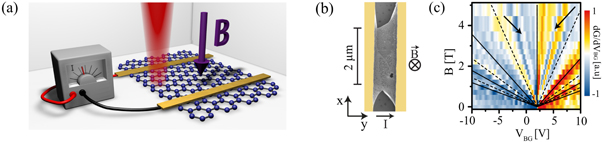
Figure 1. (a) Schematic of the photocurrent measurement. (b) Scanning electron micrograph of the suspended graphene structure, taken after the measurements. The Ti/Au contacts can be seen as yellow stripes on the left and right hand side. (c) Two-terminal transconductance as a function of the magnetic field and the gate voltage. Dotted (continuous) lines display filled (half filled) Landau levels, respectively, calculated from the Landau energy spectrum and the geometric capacitance. Two arrows show the position of additional plateaus, indicating the splitting of the zeroth level.
Download figure:
Standard image High-resolution imageApart from the high charge carrier mobility and the broad absorption bandwidth, which remains true for the edge states in a magnetic field, graphene has a number of further interesting properties for magneto-photocurrent generation. For example, the cyclotron radius of a pseudo-relativistic electronic excitation in graphene

with the elementary charge q and an energy E corresponding to, say, room temperature within a magnetic field B of 4 T (see below) is 6 nm and thus well below the mean free path. Furthermore, in addition to this classical length scale, the magnetic (Landau) length  is of the same order—which shows that quantum effects have to be taken into account. The third advantage of graphene could lie in the relatively strong Coulomb interaction: in analogy to quantum electrodynamics (QED), we can construct an effective fine-structure constant in graphene

and find that this coupling strength  is much larger than
  due to
  . Intuitively speaking, the charge carriers are much slower than the speed of light c and thus have more time to interact. These comparably strong interactions could be important for the effect of carrier multiplication discussed below. This mechanism received great attention recently: charge carriers, which are optically excited with a surplus energy, can relax by exciting electron–hole pairs, effectively turning a single photon into two or more electron–hole pairs that can drive an external circuit [5–12].
2. Results
Motivated by the predictions in [4], here we experimentally investigate the photocurrent generation in suspended graphene in a quantizing magnetic field. We start from commercially available chemical vapor deposition graphene, transferred to a 285 nm SiO2-on-Si substrate. The silicon substrate is highly doped and is used as a back gate electrode. Using photolithography and an oxygen plasma, the graphene is patterned into bars of a few μm width, see figure 1(b). Afterwards, Ti/Au (5/100 nm) electrodes are defined by electron beam lithography. The contacts cover the whole width of the graphene bars and are separated by 660 nm. In a subsequent etching step using hydrofluoric acid,  of SiO2 are removed below the graphene, which creates a suspended field-effect transistor structure [13, 14]. A scanning electron micrograph of the suspended graphene (taken after the photocurrent measurements) is shown in figure 1(b).
Our measurement setup consists of a confocal microscope inside a liquid helium cryostat, which allows us to measure at a temperature of 4.2 K and in magnetic fields of up to 9 T. After cooling down, the graphene is cleaned in-situ by a current annealing step [13, 15]. To check the quality of the graphene, we perform transconductance measurements dG/dVBG in different magnetic fields. Here G is the conductance of the graphene channel and VBG is the bias applied to the back gate to control the charge carrier density in the graphene. The resulting Shubnikov-de Haas oscillations are shown in figure 1(c). The Dirac point lies at  , so that the Landau levels fan out from this point. The expected fan diagram (dotted and solid lines in figure 1 (c)) is calculated from the geometric capacitance and the theoretical energy spectrum of single layer graphene
  , where j is the Landau level index. The good agreement with the experimental data confirms the geometric capacitance and shows that the graphene is suspended in a single layer. Furthermore, the Landau fan chart extrapolates to
  for electrons and holes, respectively, which is the fingerprint of single layer graphene (see supplemental information is available online at stacks.iop.org/NJP/19/063028/mmedia). Finally, well-developed quantum Hall plateaus confirm the quality of the investigated sample, see supplementary figure S 1. The Shubnikov-de Haas oscillations can be observed at magnetic fields as low as 0.5 T, indicating a mobility of
  [13]. At magnetic fields above 1 T, additional plateaus appear, showing at least partial splitting of the zeroth Landau level. This effect is often observed in high-quality samples and is frequently attributed to electron–electron interactions [16–18].
Next we investigate the photocurrent generation in suspended graphene. For this purpose, we use the confocal microscope and a near-infrared laser with a wavelength3
of 972 nm and a spot diameter of roughly 1.5 μm. The illumination power is 3 μW and we use a low-impedance ( ) current amplifier to directly measure the photocurrent. The laser spot is positioned in between the two gold contacts.
Figure 2(a) shows the generated photocurrent at B = 5 T, well within the quantum Hall regime. The photocurrent is found to be symmetric around the Dirac point, but there is a clear change in polarity, depending on which edge of the graphene is illuminated. This is in agreement with the magnetic-field induced chirality of the charge-carrier motion (see below).

Figure 2. (a) Photocurrent at B = 5 T as a function of the laser spot position and the gate voltage. The color scale is linear, with white corresponding to 0 nA. The solid vertical line shows the Dirac point, the dashed line indicates an empty zeroth Landau level. The picture of the graphene on the right hand side roughly indicates the position of the laser spot. (b) Photocurrent of position A at the Dirac point as a function of the magnetic field. (c) Gate voltage dependence of the photocurrent for different magnetic fields.
Download figure:
Standard image High-resolution imageWithout an applied bias, the measured photocurrent reaches surprisingly high values of over 400 nA at the Dirac point when illuminating the upper edge (position A in figure 2(a)). Considering the illumination power of 3 μW, this corresponds to a photo-responsivity of 0.13 A W−1, a value more than an order of magnitude higher than reported previously for single layer graphene devices [19, 20] and comparable to the responsivity of commercially available photodiodes.
The gate-voltage dependence of the magneto-photocurrent at different magnetic fields is shown in figure 2(c). The photocurrent at zero magnetic field (black line) features a step at the Dirac point, often observed at pn or graphene-metal junctions, and commonly attributed to thermoelectric effects [3]. For an applied magnetic field, the step at the Dirac point turns into a peak, whose height and width first increases with increasing magnetic fields but later (for  ) decreases again, see figure 2(b).
3. Discussion
Having measured such a strong magneto-photoelectric response, let us discuss possible mechanisms for generating it. Inserting the incident photon energy of 1.28 eV, we find that the observed photo-responsivity of 0.13 A W−1 corresponds to 17 electron–hole pairs per 100 incident photons. Even if we make the unrealistic assumption that the entire laser spot illuminates the suspended graphene monolayer, this value seems to contradict the standard absorption of graphene [25] of 2.3%, corresponding to less than 3 generated electron–hole pairs per 100 incident photons. In the following, we discuss possible mechanisms for this 7-fold increase.
3.1. Enhanced absorption
As one way to resolve this puzzle, one could speculate that the absorption is strongly enhanced for some reason. For example, the resonant transition between Landau levels can correspond to an effective absorption exceeding 2.3% due to a peak in the density of states (DOS) at resonance [26, 27]. E.g., [26] reports on an absorption probability of approximately 13% at 4 T for a low lying resonance (between 70 and 80 meV). However, there are several reasons why we do not believe that the measured strong magneto-photoelectric response (at 1.28 eV) is generated by such an effect.
The enhanced absorption caused by the peak in the DOS is most pronounced at resonance for low-lying bulk Landau levels with sharp energies (i.e., without dispersion). However, when sweeping the magnetic field, we did not observe resonance effects and our incident photon energy of 1.28 eV is comparably large. Furthermore, bulk Landau levels with sharp energies would not directly generate a current—whereas the observed chirality of the current points towards edge modes [20], which do show dispersion, i.e., do not have a sharp energy, see figure 3(b). Finally, for magnetic fields of 1 T, for example, the relevant Landau levels do not fit into our sample because their cyclotron radius r in equation (1) exceeds half the distance between the metal contacts4 .

Figure 3. Sketch of the proposed mechanism in real space (a) and in an energy–momentum diagram (b). In a semi-classical picture (a), after optical excitation (with  ), the generated primary charge carriers move along curved trajectories until they collide with the graphene edge (horizontal black line), at which point they can excite secondary electron–hole pairs through inelastic Coulomb scattering (governed by
  ). This Auger-type process is depicted in (b) within the energy dispersion diagram of the edge channels.
Download figure:
Standard image High-resolution imageIn appendix A.2, we present a calculation of the photon absorption into the relevant edge modes of graphene, based on linear response theory, which shows that the edge modes cannot absorb 17% of the incident laser light. In fact, the total absorption into the edge modes is somewhat reduced below 2.3%. We also estimated the near-field enhancement due to the metal contacts via a Maxwell solver (see supplemental information). Even though the electromagnetic field is affected by the presence of the metal contacts, this modification cannot account for the measured strong current.
3.2. Thermoelectric effects
As another way to explain the surprisingly large photocurrent, we consider the scenario that the laser heats up the metal contacts, which then induces thermoelectric effects at the graphene-metal junction [3]. While this effect could explain the step near the Dirac point in figure 2(c) at zero magnetic field, we are mostly interested in the peak of the current around the Dirac point at large magnetic fields (5 T, for example). The distinct dependences on gate voltage, laser polarization and laser spot position suggest that the zero-field and the large-field signals are caused by different mechanisms.
First, the broad peak of the large-field signal at the Dirac point is in strong contrast to the expected behavior (step at the Dirac point and oscillatory away from it) of usual (diffusive) thermoelectric effects in the quantum Hall regime [21–24]. Second, this large-field signal assumes its maximum for a laser polarization in y-direction (see supplemental information), while the heating of the metal contact should be most efficient for a laser polarization in the other x-direction. Third, when varying the y-position of the centre of the laser spot, the zero-field signal vanishes in the middle, where both contacts are illuminated equally strong (see supplemental information). In contrast, for high B-fields, the signal assumes its maximum in the central y-position (see supplementary figure S 4), while it changes its sign when varying the x-position of the laser, see figure 2(a), as expected for the magneto-photocurrent mechanism discussed below. Altogether, the dependence of the high magneto-photocurrent on the y-position of the laser spot centre (distance to the metal contacts) shows that it is not caused by the metal contacts while the x-dependence (distance to the edges) shows that it is an edge effect.
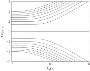
Figure A1. Dispersion relations of the edge modes in graphene with zigzag-boundary in a constant magnetic field for the lowest quantum numbers  .
.
Download figure:
Standard image High-resolution image3.3. Magneto-photocurrent
As explained above, we do not believe that the observed photo-responsivity of  at large magnetic fields can be explained by an enhancement of the absorption or the aforementioned thermoelectric effects. Thus, we consider in the following that the incident photons create a small number of primary particle–hole excitations directly—which then generate secondary particle–hole pairs via charge carrier multiplication, see figure 3. Carrier multiplication in graphene is promoted by its large effective fine-structure constant, as mentioned above. It has been theoretically predicted and experimentally observed in the past [10–12].
Since the wavelength of those primary electron or hole excitations  is much smaller than all other relevant scales, the universal absorption probability
  should be a reasonable zeroth-order approximation (see also appendix A.2). With this probability, the incident photon of energy
  eV creates a pair of an electron and a hole with equal energies of
  and opposite momenta due to energy–momentum conservation.
However, the momentum of the electron (or hole) can point in both directions with equal probability and thus no net current is generated at this stage. Since the wavelength of the electron or hole excitations  is much smaller than the classical cyclotron radius (1) of
  at 4 T, we can treat the propagation semi-classically. Thus, the electron and hole excitations describe circular trajectories with the cyclotron radius (1) until they reach the metallic contacts or they are scattered by defects or the graphene edge. A net current is induced when at least one of the carriers is reflected at the graphene edge, where the originally random direction of charge separation is transformed into a determined directionality/chirality as in figure 3, where holes move to the left and electrons to the right. The current runs into opposite directions at the upper and lower edge, which explains the position dependence in figure 2(a). This simple picture also accounts for the observed dependence on the magnetic field: if the magnetic field is too small, the radius (1) is much larger than the distance between the metallic contacts and thus the trajectories are not bent enough to control (rectify) the direction of charge separation efficiently. For intermediate field strengths of around 4 T, the circular diameter of
  fits well into the graphene sample and thus (directed) charge separation is most efficient. If the magnetic field becomes too large, however, this diameter shrinks and thus the incident photon must be absorbed very near the edge when the circle is supposed to intercept the edge—i.e., the effective absorption area shrinks.
3.4. Charge carrier multiplication
However, as explained above, these primary electron–hole pairs (directly created by the incident laser photons) cannot account for the observed current. In order to explain the generation of secondary electron–hole excitations, a natural candidate is carrier multiplication via inelastic Auger type scattering at the graphene edge. Neglecting dielectric and screening effects in our order-of-magnitude estimate, we consider the Coulomb interaction Hamiltonian

with the charge density operator  , where
  is the two-component (spinor) field operator. In principle, this nonlinear interaction Hamiltonian could also induce carrier multiplication in translationally invariant (bulk) graphene. However, this process is strongly suppressed in analogy to QED where a high-energy photon alone cannot create electron–positron pairs: when an electron is scattered inelastically from
  to
to  while creating a secondary electron–hole pair with
  and
and  , the energy–momentum conservation together with the linear dispersion relation
  implies that all these wavenumbers must be parallel
  such that the phase-space volume is basically zero. This suppression can be diminished by the coupling to phonons, defects, or a magnetic field, etc., and carrier multiplication has been observed in such scenarios [10–12, 28].
Here, we consider the inelastic reflection at the graphene fold or edge (see figure 3) where the perpendicular momentum is not conserved and thus we expect carrier multiplication effects. Via standard perturbation theory with respect to the interaction Hamiltonian (3), we calculate the probability for Auger-type inelastic scattering of a primary excitation from its initial wave function  to
to  while creating a secondary electron–hole pair with
  and
and  (see appendix A.1). Up to a dimensionless integral (which can be evaluated numerically), we find that this probability
  scales with the squared coupling constant in equation (2). Inserting realistic values, we get decay rates (probabilities per time) of several THz. As a result, the primary excitations should be able to create many secondary particle–hole pairs before reaching the metal contact—consistent with our observations.
The presented theoretical model—ranging from the creation of primary electron–hole excitations by the incident photons and their subsequent propagation on circular orbits up to the generation of secondary electron–hole excitations via inelastic (Auger-type) scattering at the graphene edge/fold, see figure 3—matches the observations, including the dependence on laser spot position and magnetic field, quite well. The gate-voltage dependence can also be understood within this picture: deviations from the Dirac point reduce the available phase space for the generation of secondary electron–hole excitations since the required energy increases. Note that only Auger-type electron–hole excitations from a downward to an upward sloping dispersion curve contribute to the net current because the current is determined [4] by the group velocity  in figure 3(b).
3.5. Conclusions
Motivated by our previous prediction [4], we have observed a surprisingly high magneto-photocurrent in suspended graphene. The observed photo-responsivity of 0.13 A W−1 corresponds to 17 electron–hole pairs per 100 incident photons, which we believe to be one of the highest values ever measured in single-layer graphene.
We discuss possible mechanisms for generating such a strong photocurrent and come to the conclusion that a theoretical model based on charge carrier multiplication via inelastic scattering of primary photo-generated excitations at the graphene edge describes the observations best. The number of created electron–hole pairs per absorbed photon ( ) exceeds most of previous observations of charge carrier multiplication in graphene as well as in any optically excited semiconductor system so far [5–12]. The effectiveness of this process can mainly be attributed to three factors:
- (a)the comparably strong Coulomb interaction quantified by
 ,
, - (b)the enlarged phase space due to the lifting of the transversal momentum conservation at the fold or edge,
- (c)the robust chiral edge states in a magnetic field, which ensure that basically all secondary carriers generated at the edge will contribute to the photocurrent.

Of course, this theoretical model is based on our current data and understanding, while more experimental and theoretical investigations are needed to fully comprehend the underlying mechanism. In any case, our findings show that graphene with its high carrier mobility and broad absorption bandwidth is a very promising material for photo-electric applications.
Acknowledgments
The authors acknowledge support by DFG (SFB-TR12 and SFB-1242).
Note added
After completing the work reported on in this manuscript, we became aware of a recent similar work on graphene–boron–nitride heterostructures by Wu et al [29].
Appendix
A.1. Estimate of carrier multiplication probability
In order to obtain a rough estimate for the carrier multiplication probability, we use first-order perturbation theory and start from the Coulomb interaction Hamiltonian (3), neglecting effects due to screening and the dielectric permittivity. In principle, one could have Coulomb interactions between different Dirac points, but here we shall focus on carrier multiplication effects within the vicinity of one Dirac point only. In this approximation, the charge density operator  is effectively given by the two-component (spinor) field operator
  . Close to the Dirac point, this effective spinor field satisfies the Dirac equation (
 )
)

with ![${x}^{\mu }=[{v}_{{\rm{F}}}t,x,y]$](https://content.cld.iop.org/journals/1367-2630/19/6/063028/revision2/njpaa739dieqn46.gif) and the Dirac matrices
and the Dirac matrices ![${\gamma }^{\mu }=[{\sigma }^{z},{\rm{i}}{\sigma }^{y},-{\rm{i}}{\sigma }^{x}]$](https://content.cld.iop.org/journals/1367-2630/19/6/063028/revision2/njpaa739dieqn47.gif) .
.
In order to specify the geometry, we consider a straight graphene edge with zigzag boundary conditions in the presence of a constant transverse magnetic field B. However, as one may infer from the arguments below, other geometries (such as a graphene fold, see [4]) yield the same order of magnitude. In the Landau gauge, the vector potential for a constant magnetic field B perpendicular to the graphene sheet adopts the form ![${A}_{\mu }=[0,0,{Bx}]$](https://content.cld.iop.org/journals/1367-2630/19/6/063028/revision2/njpaa739dieqn48.gif) . We consider a graphene sheet which is infinitely extended in the y-direction and terminated by a zigzag edge at x = 0. Then, stationarity and translational invariance in y-direction allows us to employ the separation ansatz for the (unperturbed) eigenmodes of the Dirac equation
. We consider a graphene sheet which is infinitely extended in the y-direction and terminated by a zigzag edge at x = 0. Then, stationarity and translational invariance in y-direction allows us to employ the separation ansatz for the (unperturbed) eigenmodes of the Dirac equation

where the two quantum numbers  and
and  specify the dependence on x and y, respectively. Note that the eigenenergies
  can be positive (particle states) as well as negative (hole states) and even zero (zero mode), see below. Insertion into equation (4) yields the coupled set of equations


while the zigzag boundary condition is included via the requirement  , see, e.g., [30–32]. The solutions can be expressed in terms of parabolic cylinder functions Dν via

with the index  and a suitable normalization constant
  . This index ν and thus the eigenenergy
  is determined by the zigzag boundary condition
  which implies that we must have a zero of the parabolic cylinder functions Dν at the edge where x = 0. For
  , we recover the usual bulk Landau levels with
  , while in the other limit
  , the dispersion relation becomes approximately linear
  , see figure A1.
A particular feature of the zigzag boundary condition is the appearance of a zero-energy mode. It possesses only one non-vanishing spinor component, namely ![${\psi }_{2}^{0,{k}^{y}}(x)={N}_{0,{k}^{y}}\exp (-{k}^{y}x-{x}^{2}/[2{{\ell }}_{B}^{2}])$](https://content.cld.iop.org/journals/1367-2630/19/6/063028/revision2/njpaa739dieqn61.gif) . The expansion of the field operator in terms of the (unperturbed) spinor-wavefunctions reads
. The expansion of the field operator in terms of the (unperturbed) spinor-wavefunctions reads

where  and
and  are the annihilation operators for particles (
 ) and holes (
 ), respectively, while
  corresponds to the zero mode.
In complete analogy to Fermi's golden rule, we estimate the probability (per unit time) for secondary particle–hole pair creation via time-dependent perturbation theory. The initial state  is the state of an incoming particle with
  and nin. Via inelastic Auger-type scattering at the graphene edge, this incoming particle can be reflected to an outgoing particle state with
  and nout while creating a secondary particle–hole pair with the quantum numbers
  and npart, as well as
  and nhole, respectively. Hence the final state is given by
  . To first order, the relevant matrix element is given by

The time-dependence in  reflects the unperturbed dynamics (interaction picture) from equation (4) and is encoded in the usual oscillating phase factors
  in the mode functions in equation (9).
After inserting the relevant expressions, the t-integration yields a Dirac δ-function corresponding to energy conservation (as expected)

The integrations over y and  can also be performed analytically. As usual, it is convenient to transform the variables
  and
and  to center of mass
  and distance
  coordinates. The integration over
  yields momentum conservation in y-direction while the integral over
  can be expressed in terms of the modified Bessel function of the second kind
  . Note that, for given momenta
  and
and  and quantum numbers
  , and nin, the other wavenumbers
  and
and  are fixed by the conservation of energy and momentum in y-direction.
The remaining integrals over  can be cast into a scale free form by introducing the dimensionless variables
  and analogously
  etc. In this way, the total probability per unit time (in analogy to Fermi's golden rule) can be written as

Here  denotes the dimensionless weight factor (corresponding to the DOS)

with  from equation (11). The dimensionless integrand
  represents the matrix elements in equation (10)

where the function  is decomposed of bi-linear forms of the parabolic cylinder functions in equation (8), evaluated at χ and
  , respectively.
The main point is that the decay rate (probability per unit time) in equation (12) is basically set by the characteristic frequency scale  times
times  , because the remaining integration over all final wave-numbers
  as well as the
  -integrals in
  involves only dimensionless quantities of order unity. Apart from the overlap of wave-functions which can be extremely small for certain parameters, these integrals do neither contain very small nor very large numbers which could lead to their suppression. The three remaining integrations (
 and
and  ) can be done numerically for a given set of parameters
  .
.
In order to study an explicit example, we consider a magnetic field of B = 5 T corresponding to  and
and  . As a suitable initial state, we choose
  and
and  which corresponds to an energy of
  . The decay rate of this initial state into the final states
  , and
, and  , for example, can be estimated by numerically integrating (12) and is given by

Note that this decay channel is only available if the relevant zero mode was occupied initially such that one is able to transfer an electron from this mode to the mode  , thereby creating a hole with
  . However, the decay rate for the opposite process, i.e., with
  and
and  , is nearly the same. In these processes, the zero mode acts as a reservoir for absorbing momentum (in the y-direction) without any energy cost. The probabilities for channels not involving the zero mode are somewhat smaller, e.g., for
  and
and  , we get
  for the same initial state. This suggests that phase-space arguments due to energy-momentum conservation play an important role for suppressing the carrier multiplication probability. The graphene edge lifts momentum conservation in x-direction, and thus facilitates strong carrier multiplication. Further enhancement will emerge when the phase space is also not restricted by momentum conservation in y-direction. This may result from the aforementioned zero mode or from inhomogeneities such as cracks or other defects that are typically found at the graphene edge.
If we remember that an excited particle typically spends a time of order picoseconds in the graphene sheet before reaching one of the metal contacts, we see that there is ample time for carrier multiplication. In fact, owing to the largeness of  , the above decay rate is so big that one might wonder whether first-order perturbation theory is applicable in the given situation. However, even though first-order perturbation theory may not be very accurate, one would expect that it reproduces the correct order of magnitude and shows that the probabilities are certainly not negligible. Quite analogous arguments can be applied to other geometries, such as a graphene fold, see [4], and demonstrate that the decay rates have a comparable order of magnitude—especially when the curvature radius of the fold is of the same order as
  (which is the relevant case here). Thus, even though the above derivation is based on a specific idealized geometry, the scaling arguments following equation (12) and the robustness of the chiral edge modes—which exist quite independently of the precise character of the boundary conditions at the edge or fold— indicate that other geometries yield qualitatively analogous results and the same order of magnitude.
A.2. Estimate of light absorption
In order to estimate the creation of primary charge carriers in the relevant edge modes of graphene, we treat the laser field as a classical field  . Then we may derive the generated current
  via standard time-dependent perturbation theory in first order of the interaction Hamiltonian

which gives the Kubo formula

where the unperturbed expectation value of the commutator ![$\langle [{\hat{j}}_{\nu }(t^{\prime} ,\vec{r}^{\prime} ),{\hat{j}}_{\mu }(t,\vec{r}\,)]{\rangle }_{0}$](https://content.cld.iop.org/journals/1367-2630/19/6/063028/revision2/njpaa739dieqn122.gif) is related to the conductivity tensor
is related to the conductivity tensor  . If we focus on one spin component and one Dirac point, the current density
  is related to the spinor field operator
  via
via

In analogy to equation (9), the spinor field operator  can be expanded into creation and annihilation operators multiplying the mode functions corresponding to a given scenario. If we insert the standard plane waves for planar graphene without any magnetic field, a comparison of the laser intensity
  and the absorbed energy density
  due to the generated current
  yields a photon absorption probability of
  , which—after taking into account both spin components and the two Dirac points—reproduces the well-known universal absorption probability of
  . Similarly, inserting the mode functions (and eigen-energies) of the bulk Landau levels in planar graphene with a constant magnetic field reproduces the resonant transitions between them.
Here, we insert the mode functions of the edge modes (8) as in equation (9) in order to describe the light induced excitation of edge modes, using the same values as above, i.e., B = 5 T corresponding to  and
and  . Note that the photon energy of 1.28 eV considered here is not resonant to any transitions between bulk Landau levels, such that we only have absorption into the chiral edge states (which contribute to the current). The resulting photon absorption probability as a function of distance to the edge is plotted in figure A2 for the two linear photon polarizations (parallel and perpendicular to the edge).

Figure A2. Photon absorption probability as a function of distance x to the edge for two linear laser polarizations: parallel to the edge (blue) and perpendicular to the edge (black).
Download figure:
Standard image High-resolution imageVery close to the edge, both polarizations show a peak around 3% which is caused by the zero mode  in equation (9) but can be neglected in the total integrated probability. Apart from this peak (which vanishes if we remove the zero mode) and some small scale oscillations, the probabilities start at a value of 2.3% or somewhat below at x = 0 and decrease for larger distances x until they basically vanish around
  . This is consistent with the semi-classical picture in section 3.3 since the diameter of a classical (pseudo-relativistic) circular orbit with an energy of 0.64 eV (i.e., half the photon frequency) at 5 T is around 21
  . Even the polarization dependence observed in figure A2 can be explained within this semi-classical picture, because the particle–hole pairs are predominantly emitted perpendicularly to the photon polarization. Thus, for photons absorbed very close to the edge (small x), the probability of creating an edge state (corresponding to a skipping orbit) is near unity for a laser polarization parallel to the edge, but reduced for perpendicular polarization (since the circular orbit could be directed away from the edge—which would not contribute to the current). On the other hand, for distances approaching the cyclotron diameter of around 21
  , the point where the photon is absorbed should lie close to the 'north pole' of the circular orbit (as in figure 3 (a)) in order to facilitate an edge mode (i.e., skipping orbit), which favors perpendicular polarization.
Scaling arguments very similar to those in the previous section A.1 show that other geometries (such as a graphene fold [4]) or boundary conditions (such as armchair) lead to analogous behavior and the same orders of magnitude, even though the details (e.g., selection rules regarding the photon polarization, see [4]) can be different.
Footnotes
- 3
The photon energy of 1.28 eV is chosen such that it is much larger than the typical Landau level energy
but still small enough such that the linear (pseudo-relativistic) dispersion relation is a good approximation. - 4
Note that the wave functions of the bulk Landau levels (corresponding to full circular orbits) are more spread out than those of the chiral edge states, which correspond to skipping orbits (see figure 3(a)) containing circular segments only and thus can be much more localized. Hence, even if bulk Landau levels do not fit into our sample, it can still support chiral edge states.

