Time averaging, ageing and delay analysis of financial time series

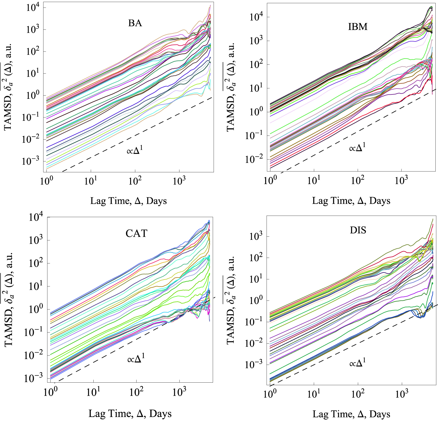
For sufficiently long time series the time averaged MSD (1) typically produces relatively smooth results as a function of lag time. This feature is immediately obvious from the plots of $\overline{{\delta }^{2}({\rm{\Delta }})}$ for data shown in figure 2. We emphasise that in the calculation of the time averaged MSD, for any given lag time Δ the entire time series is used and thus the initial values X₀ always contribute to the magnitude of $\overline{{\delta }^{2}({\rm{\Delta }})}$. The lag time increment is 10 days in figure 2, and we used the 'raw' time series in this analysis (no normalisation to X(t) values at the initial or final point is performed). Shorter lag times are computationally more expensive but would allow for a better resolution of the initial growth of $\overline{{\delta }^{2}({\rm{\Delta }})}$. The spread of the computed magnitudes of $\overline{{\delta }^{2}({\rm{\Delta }})}$ at short lag times increases with T for growing stock market prices, as long as no market crises occur, as seen in figure 2.

Zoom In Zoom Out Reset image size

We observe a roughly linear growth $\overline{{\delta }^{2}({\rm{\Delta }})}\propto {\rm{\Delta }}$ at short lag times, in perfect accordance with the analytical result (6) for GBM derived below. This linear scaling stands in stark contrast to the exponential growth of the ensemble averaged MSD $\langle {X}^{2}(t)\rangle$ of GBM seen in equation (5) below. Such a fundamental discrepancy between the time and ensemble averaged MSD of the process X(t) is well known in the theory of stochastic processes and often referred to as weak ergodicity breaking [55, 56]. For financial time series the fact that $\overline{{\delta }^{2}({\rm{\Delta }})}\propto {\rm{\Delta }}$ allows the direct analysis of X(t) instead of its logarithm.

When the lag time approaches the length T of the time series, it is obvious from definition (1) that the statistic is worsening. This intrinsic property of time averages is reflected by the increasing fluctuations of $\overline{{\delta }^{2}({\rm{\Delta }})}$ seen in figure 2. Note that in the limit ${\rm{\Delta }}\to T$ the time-ensemble averaged MSD, averaged over N independent trajectories of the same process, under identical starting conditions and parameters,

$$\begin{eqnarray}&&\phantom{\rule{}{.25ex}}\langle \overline{{\delta }^{2}({\rm{\Delta }})}\phantom{\rule{}{.25ex}}\rangle =\displaystyle \frac{1}{N}\displaystyle \sum _{i=1}^{N}\overline{{\delta }_{i}^{2}({\rm{\Delta }})},\end{eqnarray} \tag{ 2 }$$

is equal to $\langle {[X(t)-{X}_{0}]}^{2}\rangle$ [55]. Note that the averaging over different trajectories in quantity (2) is necessary for our analytical calculations. In the analysis of the financial time series shown in the figures, single trajectory averages $\overline{{\delta }^{2}({\rm{\Delta }})}$ are considered throughout.

Before continuing with our analysis of the actual stock market data, we briefly digress and provide a primer on GBM, a paradigm process employed in standard models for stock price dynamics. As we show this model reproduces the essential features observed in the market data.

GBM is defined in terms of the stochastic differential equation with multiplicative noise

$$\begin{eqnarray}&&{\rm{d}}{X}(t)=\mu X(t){\rm{d}}{t}+\sigma X(t){\rm{d}}{W}(t).\end{eqnarray} \tag{ 3 }$$

Here $X(t)\gt 0$ is the price at time t, μ denotes a drift, and σ is the volatility (μ and σ are set constant below). The volatility is connected to the square root of the diffusivity [55]. The increments dW of the Wiener process $W(t)={\int }_{0}^{t}\xi (t^{\prime} ){\rm{d}}{t}^{\prime}$ are defined as white Gaussian noise $\xi (t)$ with zero mean. The price evolution, starting with the initial value ${X}_{0}\gt 0$ at t = 0, is obtained from equation (3) by use of Itô's lemma [12, 14] as

$$\begin{eqnarray}&&X(t)={X}_{0}{{\rm{e}}}^{(\mu -{\sigma }^{2}/2)t+\sigma W(t)}.\end{eqnarray} \tag{ 4 }$$

This process satisfies the log-normal distribution, emerging also in models of task success and income distribution [57]. The MSD shows the exponential growth

$$\begin{eqnarray}&&\langle X{(t)}^{2}\rangle ={X}_{0}^{2}{{\rm{e}}}^{(2\mu +{\sigma }^{2})t}.\end{eqnarray} \tag{ 5 }$$

Due to this (much) faster growth compared to the linear increase of the MSD with t for Brownian motion, GBM is therefore a superdiffusive process [55].

To calculate the time averaged properties of interest, we resort to the average (2) over N independent realisations of X(t). We derive this quantity using the one and two point distribution functions of the Wiener process. For short lag times, ${\rm{\Delta }}\ll T$, and in the absence of drift we find

$$\begin{eqnarray}&&\phantom{\rule{}{.25ex}}\langle \overline{{\delta }^{2}({\rm{\Delta }})}\phantom{\rule{}{.25ex}}\rangle \sim {X}_{0}^{2}({{\rm{e}}}^{{\sigma }^{2}T}-1)\displaystyle \frac{{\rm{\Delta }}}{T}\sim \langle X{(T)}^{2}\rangle \displaystyle \frac{{\rm{\Delta }}}{T}.\end{eqnarray} \tag{ 6 }$$

As mentioned already, the non-equivalence of the ensemble and time averaged MSD, $\langle {X}^{2}({\rm{\Delta }})\rangle \ne \langle \overline{{\delta }^{2}({\rm{\Delta }})}\rangle$ in the limit ${\rm{\Delta }}/T\ll 1$ indicates weak ergodicity breaking, known for other non-stationary diffusion processes [55]. The time averaged MSD (6) scales linearly with the lag time Δ, in contrast to the exponential growth of $\langle X{(t)}^{2}\rangle$, but grows exponentially with the trace length T, due to the highly non-stationary character of GBM.

We now return to the discussion of the time averaged MSD of the different stocks. The time averaged MSD of the analysed financial time series, similar to equation (6) for the GBM process, is expected to be a growing function of the trajectory length T. Indeed, this behaviour is demonstrated in figure 2, in which we plot the time averaged MSD $\overline{{\delta }^{2}({\rm{\Delta }})}$ for varying trace length T for four different stock prices. This fact mirrors the accelerating nature of the stochastic process underlying the price variations.

What happens when the index value stagnates or drops substantially within a prolonged period of time, as can be seen in figure 1 following the 2008–2009 crisis? In this case the time averaged MSD $\overline{{\delta }^{2}({\rm{\Delta }})}$ evaluated for partial time series (different T values) encompassing this time window tend to cluster together. Consequently, the value of $\overline{{\delta }^{2}({\rm{\Delta }})}$ may saturate in this region, compare the original tick data in figure 1, the behaviour of $\overline{{\delta }^{2}({\rm{\Delta }})}$ versus lag time Δ in figure 2, and the explicit dependence on T shown in figure 3.

Zoom In Zoom Out Reset image size

Equation (6) predicts, to leading order, an exponential growth of the time-ensemble averaged MSD with the trace length T. As shown in figure 3, computed for ${\rm{\Delta }}=1$ day, the data indeed roughly follow an exponential increase with T. However, no universal dependence of the time averaged MSD as function of T could be found. Especially for those time windows encompassing prolonged drops or stalling of the index price, the ratio of the time averaged MSD for a trace length T to its value at ${T}_{\min }$ does not grow rapidly but rather saturates, as can also be seen in figure 3. Thus, checking the dependence of $\overline{{\delta }^{2}({\rm{\Delta }})}$ on the trace length T may be used to unveil individual features of index price dynamics. In contrast to the strongly disparate and company-specific behaviour revealed in figure 3, universal features are found in the analysed index prices when employing the new concept of the delay time averaged MSD introduced below.

Figure 4 shows the data normalised to their end point. More specifically, this normalisation $\overline{{\delta }_{n}^{2}({\rm{\Delta }})}\sim {X}_{n}^{2}(T)({\rm{\Delta }}/T)$ enhances the contribution of later parts of the time series, with typically larger prices. We find a considerable spread of individual $\overline{{\delta }_{i,n}^{2}}$ traces for different companies, because each index can have different parameters such as the volatility value or the attitude of a given company leadership to maximise the short-term profit versus ensuring a long-time sustainability. Finite lifetimes of companies and their varying age at the start of the time series are likewise important. These factors individualise stock price variations for each company and complicate the evaluation of ensemble averaged quantities. In view of this the universality of stock prices observed in section 2.5 is even more remarkable.

Zoom In Zoom Out Reset image size

Physically, the above dependence (6) of the time averaged MSD on the trace length T reflects the phenomenon of ageing, a characteristic property of non-stationary stochastic processes [55, 58]. For superdiffusive processes with an MSD growing faster than the linear growth in time of Brownian motion, the time averaged MSD exhibits an increase with T. This reflects the self-reinforcing volatility of the process, as seen for the exponentially fast growth in equation (6). In contrast, in subdiffusion the effective diffusivity of the process is a decaying function of time [55]. For instance, in processes with scale free waiting times the typical sojourn periods of the motion become increasingly long, on average, effecting the decay of the time averaged MSD with T [58].

Another way to analyse ageing processes is the following. If the time series X(t), starting at time t = 0, is evaluated only beginning with the so-called ageing time ${t}_{{\rm{a}}}\gt 0$, the ageing time averaged MSD is defined as [58]

$$\begin{eqnarray}&&\overline{{\delta }_{{\rm{a}}}^{2}({\rm{\Delta }})}=\displaystyle \frac{1}{T-{\rm{\Delta }}}{\int }_{{t}_{{\rm{a}}}}^{{t}_{{\rm{a}}}+T-{\rm{\Delta }}}{[X(t+{\rm{\Delta }})-X(t)]}^{2}{\rm{d}}{t}.\end{eqnarray} \tag{ 7 }$$

In this formal definition we shift the starting point for the analysis of the time series yet the length T of the analysed time interval remains fixed. Of course, larger values of t_a limit the remaining number of data points available for this analysis, however, the ageing time averaged MSD provides important insights into the underlying stochastic process [55]. We note that the term ageing does not imply any relaxation to an ergodic state in the limit of long ageing times, as it does for subdiffusive processes (the limit of strong ageing). In superdiffusive processes such as GBM and, as shown here, for highly non-stationary financial data the term ageing delineates the process time dependent increase of the spread of the random variable X(t).

For GBM we find in the limit of short lag times, ${\rm{\Delta }}\ll T$, and in absence of a drift, $\mu =0$, that on average

$$\begin{eqnarray}&&\phantom{\rule{}{.25ex}}\langle \overline{{\delta }_{{\rm{a}}}^{2}({\rm{\Delta }})}\phantom{\rule{}{.25ex}}\rangle \sim \phantom{\rule{}{.25ex}}\langle \overline{{\delta }^{2}({\rm{\Delta }})}\phantom{\rule{}{.25ex}}\rangle {{\rm{e}}}^{{\sigma }^{2}{t}_{{\rm{a}}}}.\end{eqnarray} \tag{ 8 }$$

The exponential growth with t_a emerges as the process X(t) already experienced an acceleration of the price dynamics up to the ageing time t_a, and thus the analysis starts with a higher volume. Note that in result (8) the argument of the exponential includes the volatility term ${\sigma }^{2}$ of the GBM process.

To see whether such ageing effects can indeed be observed in real financial data we study the behaviour of the ageing time averaged MSD $\overline{{\delta }_{{\rm{a}}}^{2}({\rm{\Delta }})}$ as function of the ageing time t_a. The raw data variation of $\overline{{\delta }_{{\rm{a}}}^{2}({\rm{\Delta }})}$ as function of the ageing time t_a for a number of indices is shown in figure 5. Indices growing rapidly and continuously in value reveal pronounced ageing effects, and $\overline{{\delta }_{{\rm{a}}}^{2}({\rm{\Delta }})}$ increases fast with t_a. Similar to the observations above, when we varied the trace length T, partial clustering of the traces for varying t_a is visible.

Zoom In Zoom Out Reset image size

Figure 6 quantifies the behaviour of the logarithm of the ratio $\overline{{\delta }_{{\rm{a}}}^{2}({\rm{\Delta }})}/\overline{{\delta }^{2}({\rm{\Delta }})}$ of the ageing time averaged MSD to the corresponding non-ageing value, plotted versus the ageing time t_a. Although, again, a roughly exponential increase is evident and consistent with the prediction (8) for GBM, no data collapse onto a universal curve is observed. Even at short ageing times we find a substantial spread of the $\mathrm{log}[\overline{{\delta }^{2}({\rm{\Delta }})}/\overline{{\delta }^{2}({\rm{\Delta }})}]$ curves versus t_a for different stock indices, as can be seen in figure 6. The non-universal behaviour is expected to be due to the fact that the volatility parameter varies between companies, as equation (8) predicts, and thus no data collapse in the growth of $\mathrm{log}[\overline{{\delta }_{{\rm{a}}}^{2}({\rm{\Delta }})}/\overline{{\delta }^{2}({\rm{\Delta }})}]$ with the ageing time t_a occurs. No averaging over different companies is performed for the ageing time averaged MSD to compute the mean value $\langle \overline{{\delta }_{{\rm{a}}}^{2}({\rm{\Delta }})}\rangle$ in figure 6 because the corresponding ensemble is not formed from trajectories with identical parameters. For instance, the volatility values and the effect of the ageing time t_a for each stock market index can be markedly different.

Zoom In Zoom Out Reset image size

What if we allow the length of the time series to vary in the above ageing analysis? Namely, what would the expected behaviour be for the quantity

$$\begin{eqnarray}&&\overline{{\delta }_{{\rm{d}}}^{2}({\rm{\Delta }})}=\displaystyle \frac{1}{T-{t}_{{\rm{d}}}-{\rm{\Delta }}}{\int }_{{t}_{{\rm{d}}}}^{T-{\rm{\Delta }}}{[X(t+{\rm{\Delta }})-X(t)]}^{2}{\rm{d}}{t},\end{eqnarray} \tag{ 9 }$$

in which we call t_d the delay time, and the trace X(t) is evaluated in the interval from $t={t}_{{\rm{d}}}$ until t = T. As long as the lag times Δ are short compared to the time span $T-{t}_{{\rm{d}}}$ of the data, it can be shown that the mean delay time averaged MSD follows

$$\begin{eqnarray}&&\phantom{\rule{}{.25ex}}\langle \overline{{\delta }_{{\rm{d}}}^{2}({\rm{\Delta }})}\phantom{\rule{}{.25ex}}\rangle \sim \displaystyle \frac{{\rm{\Delta }}}{T-{t}_{{\rm{d}}}}{X}_{0}^{2}({{\rm{e}}}^{{\sigma }^{2}T}-{{\rm{e}}}^{{\sigma }^{2}{t}_{{\rm{d}}}}).\end{eqnarray} \tag{ 10 }$$

For the ratio of the delay time averaged MSD (10) to the time averaged MSD (2) in the limit of short delay times ${t}_{{\rm{d}}}/T\ll 1$ and long traces we get the simple, parameter-free result,

$$\begin{eqnarray}&&\mathrm{log}\phantom{\rule{}{.25ex}}[\phantom{\rule{}{.25ex}}\langle \overline{{\delta }_{{\rm{d}}}^{2}({\rm{\Delta }},{t}_{{\rm{d}}})}\phantom{\rule{}{.25ex}}\rangle /\phantom{\rule{}{.25ex}}\langle \overline{{\delta }^{2}({\rm{\Delta }})}\phantom{\rule{}{.25ex}}\rangle \phantom{\rule{}{.25ex}}]\,\sim \,{t}_{{\rm{d}}}/T.\end{eqnarray} \tag{ 11 }$$

The logarithm here cancels the leading exponential dependence of the delayed time averaged MSD on t_d in equation (10) and the final result (11) is independent on the index-specific volatility parameter σ. We emphasise that in this result it is crucial that the process X(t) has non-stationary increments. The behaviour of, say, a standard Brownian process would follow a different scaling law with the delay time. Can this universal behaviour predicted in equation (11) indeed be seen in real financial time series, on the single trajectory level?

Pronounced up and down trends in the price evolution of an index give rise to strong variations of the $\overline{{\delta }_{{\rm{d}}}^{2}({\rm{\Delta }})}$ magnitudes, see figure 7. For longer t_d, the delay time averaged MSD includes a progressively shorter interval, causing a worsening statistic. Also, the magnitude of $\overline{{\delta }_{{\rm{d}}}^{2}({\rm{\Delta }})}$ increases because windows with higher prices and larger price variations are being processed in the averaging (9). For longer delay times t_d—when later parts of the time series contribute stronger to the time averaged MSD—the magnitude of $\overline{{\delta }_{{\rm{d}}}^{2}({\rm{\Delta }})}$ increases nearly linearly at short and moderate Δ, see figure 7. After a significant drop of stock index prices as a consequence of the 2008–2009 financial crisis, the variation of $\overline{{\delta }_{{\rm{d}}}^{2}({\rm{\Delta }})}$ with the delay time t_d exhibits large fluctuations for the lag times values encompassing this period of the time series. Due to this, the growing trend of $\overline{{\delta }_{{\rm{d}}}^{2}({\rm{\Delta }})}$ with the delay time may be reversed, see figure 7.

Zoom In Zoom Out Reset image size

Figure 8 shows the logarithm of the ratio of the delay time averaged MSD to the standard time averaged MSD, evaluated at unit lag time ${\rm{\Delta }}=1$, as function of the delay time t_d. The universal behaviour (11) expected on average is followed very closely for each stock market time series. This universal behaviour—fulfilled for delay times t_d up to some 5–10 years—is the central result of this study. To our best knowledge, in terms of single time series this universal trend has not been reported before.

Zoom In Zoom Out Reset image size

At longer delay times, we observe a distinct crossover to a somewhat steeper t_d-dependence in figure 8, consistent with a law of the form

$$\begin{eqnarray}&&\mathrm{log}[\overline{{\delta }_{{\rm{d}}}^{2}({\rm{\Delta }},{t}_{{\rm{d}}})}/\overline{{\delta }^{2}({\rm{\Delta }})}]\simeq {({t}_{{\rm{d}}}/T)}^{\nu }\end{eqnarray} \tag{ 12 }$$

with the scaling exponent $\nu \gt 1$. The observed behaviour features two relatively similar exponents: at short and intermediate delay times $\nu \approx 1$ while for long delay times $\nu \approx 1.3$. The initial linear scaling is universal, compare top and bottom panels of figure 8 with starting dates 1980 and 1962, respectively. As shown by the thin dashed line in the upper panel of figure 8, the second regime with $\nu \gt 1$ is more pronounced for the data starting ${t}_{0}=1980$, while it is less obvious for the ${t}_{0}=1962$ data. For long delay times we however consistently observe a faster than exponential growth of the ratio $\overline{{\delta }_{{\rm{d}}}^{2}({\rm{\Delta }},{t}_{{\rm{d}}})}/\overline{{\delta }^{2}({\rm{\Delta }})}$. In particular, this disqualifies the predictions of GBM in this long delay time regime. Note that since the time averaged MSD initially grows approximately linearly with Δ, as one can see figures 2 and 7, the trends of figure 8 will also hold for other sufficiently short lag times.

Note that for some high tech companies and banks we did not observe a growth of $\overline{{\delta }_{{\rm{d}}}^{2}({\rm{\Delta }}=1,{{t}}_{{\rm{d}}})}/\overline{{\delta }^{2}({\rm{\Delta }}=1)}$ with the delay time t_d (not shown). We believe that this is due to the very limited lengths of the time series available, starting in about 1987–1988. Therefore, effects of severe price drops during the 2008–2009 crisis dominate the magnitude of $\overline{{\delta }_{{\rm{d}}}^{2}}$ over the entire time range we examined, rendering the result (11) for the standard GBM inapplicable. For a number of German DAX companies, with time series available from 2001, the prediction (12) does not hold either (not shown).