Resonance beyond frequency-matching: multidimensional resonance

Resonance is a universal property of oscillations in both classical and quantum physics [1, 2]. It occurs at a wide range of scales, from subatomic particles [2, 3] to astronomical objects [4]. A thorough understanding of resonance is crucial for related fundamental researches [4–8] and applications [9–12]. The simplest resonance system, such as a pendulum, has one oscillating element and features a single inherent resonance frequency. More commonly, a resonator contains interacting elements and has multiple resonance frequencies. Each resonance frequency corresponds to a normal mode [1] that is characterized by unique spatial variation of the oscillation amplitude and phase. There have been extensive studies on the tunability of resonance frequency and the accessibility of local modes by geometrical means in artificial nanostructures [6, 7, 12, 13], while the spatial feature of the normal modes receives little attention.

To date, in the conventional definition of resonance, the only criterion is whether the temporal frequency of the external stimulus is equal to one of the resonance frequencies of the system, and the spatial character is ignored. Since frequency describes the periodic pattern of oscillation in the time domain, we choose to use a more specific term 'temporal resonance' for such defined phenomena. Here we reveal the generation of spatial resonance, i.e. resonance in the space domain, when we align the spatial distribution of the external stimulus with the space pattern of a normal mode. The complete resonance, which we call multidimensional resonance, must incorporate both temporal and spatial resonance. Temporal resonance alone has low capability of stimulating all modes but the fundamental one, as a result of neglecting the space variables. In contrast, multidimensional resonance is efficient for all normal modes and can be several orders stronger in magnitude.

We conduct analytical derivations and micromagnetic simulations (see appendix A) on the behavior of elastic waves in a two-dimensional circular membrane and spin waves in a ferromagnetic nanodisc, respectively. The interplay between spin waves and magnetization reversal in small magnetic structures is of particular interest to high-speed data storage devices [14–16] and logic circuits [17–20]. In ferromagnetic nanodiscs a unique spiral spin configuration called vortex state [21–23] is favorable due to the competition between magnetostatic and exchange interactions. The magnetization at the vortex core can point either upwards (polarity p = +1) or downwards (p = −1); so, a magnetic vortex can be used as a data storage element carrying one bit of information. Three classes of spin wave modes, namely gyrotropic [24], azimuthal and radial [25–28], have been discovered in magnetic discs. We focus on the radial spin wave mode of a ferromagnetic disc because it is analogous to the radially symmetric mode [29] in a two-dimensional elastic membrane, thus facilitating direct comparison.

Our calculations demonstrate spatial resonance in both the magnetic and mechanical resonators under the space-pattern-matching condition. This suggests that spatial resonance does not depend on material and, similar to the temporal resonance, is a universal property of oscillation systems. We also show that multidimensional resonance drives markedly stronger radial spin waves than does temporal resonance alone and increases the core reversal speed by more than 500%. Additional results for mechanical and magnetic strings are presented in appendices B and C, respectively, as demonstrations of multidimensional resonance in spatially one-dimensional systems.

Consider the forced small amplitude vibrations of a membrane stretched in a rigid circular frame; the equation of motion is given by [29, 30]

$$\begin{eqnarray}&&\displaystyle \frac{{\partial }^{2}W}{\partial {t}^{2}}-{a}^{2}{{\rm{\nabla }}}^{2}W=\displaystyle \frac{p(\rho ,\varphi ,t)}{\tilde{\rho }}=g(\rho )\cos \,m\varphi \,\sin \,kat.\end{eqnarray} \tag{ 1 }$$

Here, ∇² is the Laplace operator, $W(\rho ,\varphi ,t)$ is the vertical displacement of a membrane with radius ρ₀ and mass per unit area $\tilde{\rho },$ $a=\sqrt{T/\tilde{\rho }}$ is the propagation velocity of the transverse waves, and T is the isotropic tension in the membrane with dimensions of force per unit length. To facilitate discussing the efficiency of different driving forces (both spatially and temporally), the external force acting normal to the membrane is assumed to have surface density $p(\rho ,\varphi ,t)$ taking the form of the right side of equation (1) and subject to normalization condition $\displaystyle {\int }_{0}^{2\pi }\displaystyle {\int }_{0}^{{\rho }_{0}}| g(\rho )\cos \,m\varphi | \rho {\rm{d}}\rho {\rm{d}}\varphi =c\pi {\rho }_{0}^{2},$ where c is a constant.

For a stretched membrane initially at rest, the initial conditions are $W(\rho ,\varphi ,0)=0$ and ${[\partial W/\partial t]}_{t=0}=0,$ whereas the boundary conditions are $W({\rho }_{0},\varphi ,t)=0$ and ${[\partial W/\partial t]}_{\rho ={\rho }_{0}}=0.$ The solution to equation (1) satisfying these initial-boundary value conditions is obtained by separation of variables, with the result

$$\begin{eqnarray}&&W(\rho ,\varphi ,t)=\displaystyle \frac{\cos \,m\varphi }{a}\displaystyle \sum _{n=1}^{\infty }\displaystyle \frac{{J}_{m}({k}_{n}^{(m)}\rho )}{{k}_{n}^{(m)}}{I}_{n}{L}_{n}(t),\end{eqnarray} \tag{ 2 }$$

in which

$$\begin{eqnarray}&&{I}_{n}=\displaystyle \frac{2}{{\rho }_{0}^{2}{[{J}_{m+1}({k}_{n}^{(m)}{\rho }_{0})]}^{2}}\displaystyle {\int }_{0}^{{\rho }_{0}}g(\rho ){J}_{m}({k}_{n}^{(m)}\rho )\rho {\rm{d}}\rho \end{eqnarray} \tag{ 3 }$$

and

$$\begin{eqnarray}&&{L}_{n}(t)=\displaystyle {\int }_{0}^{t}\sin \,ka\tau \,\sin \,{k}_{n}^{(m)}a(t-\tau ){\rm{d}}\tau .\end{eqnarray} \tag{ 4 }$$

Here, ${J}_{m}(x)$ is the Bessel function of the first kind of order m, ${k}_{n}^{(m)}={x}_{n}^{(m)}/{\rho }_{0},$ and ${x}_{n}^{(m)}$ is the nth non-negative root of ${J}_{m}(x).$ Expression (2) shows that the stimulated vibration is a superposition of the normal modes ${J}_{m}({k}_{n}^{(m)}\rho )\cos \,m\varphi ,$ as indicated by spatial pattern index (n, m), where $n=\mathrm{1,}\,2,\ldots ,\infty$ and $m=0,1,\,\ldots ,\,\infty .$ The normal modes are determined by the resonator's geometry and boundary conditions. ${J}_{m}(x)$ changes in sign whenever $x$ moves across a node at ${x}_{n}^{(m)},$ resulting in phase reversal. The angular factor of the normal mode, $\cos \,m\varphi ,$ has opposite signs on either side of the nodal lines at $\varphi =\pm \pi /2m,\pm 3\pi /2m,\ldots ,\,\pm (2m-1)\pi /2m.$ Thus, space can be partitioned into phase zones by nodal lines, forming a space pattern that is unique to the index (n, m), see figure 1(a).

Zoom In Zoom Out Reset image size

Now, we turn to micromagnetic simulations on the radial spin wave mode of a 300 nm diameter (R = 150 nm) and 5 nm thick (L = 5 nm) permalloy (Ni₈₀Fe₂₀) nanodisc. In the static state, the disc forms a vortex state (figure 2(a)) with core polarity +1. We apply a sinc function field, expressed as ${H}_{{\rm{sinc}}}=A\,\sin [2\pi {\nu }_{{\rm{c}}}(t-{t}_{0})]/2\pi {\nu }_{{\rm{c}}}(t-{t}_{0})$ with A = 50 Oe, ν_c = 100 GHz and t₀ = 1 ns, over the entire disc to excite spin waves of all frequencies up to 100 GHz. The resulting temporal oscillation of the z-component magnetization averaged over the whole disc, 〈m_z〉, is given in figure 2(b). Next, we perform fast Fourier transform (FFT) of 〈m_z〉 to obtain the amplitude spectrum in the frequency domain [27, 31, 32]. Seven primary peaks corresponding to radial modes (n = 1, 2, ..., 7) appear at resonant frequencies of ν_n = 6.8, 9.8, 12.6, 15.9, 19.6, 24.0 and 29.0 GHz (figure 2(c)). These agree well with the experiment in [28]. For the first three radial modes, the experimental results, for this sample aspect ratio L/R = 0.033, are about 20% lower than ours as expected, because saturation magnetization of their samples is 20% smaller than the normal value of 800 KA m⁻¹ used in our numerical calculations. For higher modes, direct comparison between samples with same aspect ratio is inappropriate because the magnetostatic energy remains dominant for the micron sized samples in the experiment while both magnetostatic and exchange energy are significant for our nanometer scale sample. In the FFT-amplitude spatial distribution diagrams for the first four normal modes (figure 2(d) upper panels), we see clear quantization of the spin wave, and the number of nodes along radial direction corresponds to the mode index n. In the FFT phase diagrams for these modes (figure 2(d) lower panels), we observe high spatial uniformity for n = 1 but phase discontinuity of π across nodal lines for n > 1. Therefore, the entire sample can be partitioned into ring-shaped phase zones similar to the case of the membrane.

Zoom In Zoom Out Reset image size

We first theoretically establish the spatial resonance in the elastic membrane. Because expression (3) means the projection of g(ρ) on each mode shape ${J}_{m}({k}_{n}^{(m)}\rho )$ and because g(ρ) denotes the radial distribution of the driving force, I_n implies space-domain resonance in the radial dimension, when g(ρ) matches the space pattern of ${J}_{m}({k}_{n}^{(m)}\rho ).$ Similarly, expression (4) for L_n(t) is the convolution of the temporal variations of the driving force and the generated wavelet (i.e., a response to stimulation in the time domain) and implies time-domain resonance. A higher degree of similarity between the response and stimulation as functions of time gives rise to a larger convolution L_n(t), which is given by

$$\begin{eqnarray}{L}_{n}(t)=\left\{\begin{array}{lll}\displaystyle \frac{k\,\sin \,{k}_{n}^{(m)}at-{k}_{n}^{(m)}\,\sin \,kat}{a(k+{k}_{n}^{(m)})(k-{k}_{n}^{(m)})} & {\rm{if}} & k\ne {k}_{n}^{(m)},\\ -\displaystyle \frac{t\,\cos \,{k}_{n}^{(m)}at}{2}+\displaystyle \frac{\sin \,{k}_{n}^{(m)}at}{2{k}_{n}^{(m)}a} & {\rm{if}} & k={k}_{n}^{(m)};\end{array}\right.\end{eqnarray} \tag{ 5 }$$

thus, only temporal resonance causes a time accumulation effect.

For a spatially uniform stimulus with conventional (temporal) resonance, i.e., m = 0 and $p(\rho ,\varphi ,t)/\tilde{\rho }=c\,\sin \,{k}_{{n}_{0}}^{(0)}at,$ we have ${I}_{n}=2c/[{x}_{n}^{(0)}{J}_{1}({x}_{n}^{(0)})].$ Then, the energy in the membrane grows as

$$\begin{eqnarray}&&E=\displaystyle {\int }_{0}^{2\pi }\displaystyle {\int }_{0}^{{\rho }_{0}}\tilde{\rho }{(\partial W/\partial t)}^{2}\rho {\rm{d}}\rho {\rm{d}}\varphi =\tilde{E}{[2/{x}_{{n}_{0}}^{(0)}]}^{2}+{\rm{H}}{\rm{F}}{\rm{\text{OTs}}},\end{eqnarray} \tag{ 6 }$$

where $\tilde{E}=(\pi {\rho }_{0}^{2}\tilde{\rho }{c}^{2}/8){t}^{2}(1-\,\cos \,2{k}_{{n}_{0}}^{(0)}at),$ and the high frequency oscillating terms (HFOTs) determine fine structure of the energy curve with no influence on its general trend. Table 1 shows that the energy growth rate quickly drops for larger n₀ as $E/\tilde{E}\approx 4/{[\pi ({n}_{0}-1/4)]}^{2}$ because the stimulus, which is uniform in space and has the spatial pattern index (1, 0), is spatially off-resonance with pattern (n₀, 0) when n₀ ≠ 1; and is farther away from spatially resonant for larger n₀, although they are all temporally resonant.

Table 1.  Membrane energy growth for different stimulus in expressions (6), (7), (10) and (11).

n0	1	2	3	4	5	6	7	8	9	∞
$E/\tilde{E}$ in (6)	0.692	0.131	0.0534	0.0288	0.0179	0.0122	0.008 89	0.006 74	0.005 29	0
$E/\tilde{E}$ in (7)	1.445	1.404	1.396	1.393	1.392	1.391	1.390	1.390	1.389	1.388
$E/\tilde{E}$ in (10)	3.710	2.838	2.615	2.515	2.457	2.420	2.395	2.376	2.361	2.250
$E/{\tilde{E}}^{(1)}$ in (11)	1.535	1.634	1.664	1.678	1.687	1.692	1.696	1.699	1.701	1.712

For a radially symmetric stimulus taking the spatial resonance into consideration, for example, m = 0 and $p(\rho ,\varphi ,t)/\tilde{\rho }=(c/{s}_{{n}_{0}}){J}_{0}({k}_{{n}_{0}}^{(0)}\rho )\sin \,{k}_{{n}_{0}}^{(0)}at,$ the normalization condition demands ${s}_{{n}_{0}}=2{[{x}_{{n}_{0}}^{(0)}]}^{-2}{\sum }_{i=1}^{{n}_{0}}\displaystyle {(-1)}^{i-1}{h}_{i},$ where ${h}_{i}={x}_{i}^{(0)}{J}_{1}({x}_{i}^{(0)})-{x}_{i-1}^{(0)}{J}_{1}\,({x}_{i-1}^{(0)})$ (see figure 1(b) for n₀ = 2). Then, I_n equals $c/{s}_{{n}_{0}}$ if n = n₀ and 0 if n ≠ n₀, which shows that a stimulus tends to generate a wave similar to itself and that the normal modes are mutually orthogonal. Hence, the energy in the membrane grows as

$$\begin{eqnarray}&&E=\tilde{E}{[{J}_{1}({x}_{{n}_{0}}^{(0)})/{{s}}_{{n}_{0}}]}^{2}+{\rm{\text{HFOT}}}{\rm{s}}.\end{eqnarray} \tag{ 7 }$$

Table 1 shows that the energy grows at similar rates for different n₀ (limiting at $E=1.388\tilde{E}$ for large n₀). In this case, the stimulus has spatial pattern index (n₀, 0) and is on-resonance with space pattern (n₀, 0). The energy growth expressed by equation (7) is at least one order of magnitude larger than that expressed by equation (6), since the latter case is spatially off-resonant for n₀ > 1.

It is technically difficult to set the driving force varying as a Bessel function in the radial dimension. For ease of implementation, we employ a delta-function-like stimulus as follows

$$\begin{eqnarray}&&\displaystyle \frac{p(\rho ,\varphi ,t)}{\tilde{\rho }}=\displaystyle \frac{c{\rho }_{0}^{2}}{{s}_{{n}_{0}}{[{x}_{{n}_{0}}^{(0)}]}^{2}}\displaystyle \sum _{i=1}^{{n}_{0}}{h}_{i}\displaystyle \frac{\delta (\rho -{\rho }_{i})}{\rho }\,\cos \,m\varphi \,\sin \,{k}_{{n}_{0}}^{(m)}at,\end{eqnarray} \tag{ 8 }$$

where ${\rho }_{i}={\rho }_{0}({X}_{i}^{(m)}/{x}_{{n}_{0}}^{(m)}),$ ${X}_{i}^{(m)}$ is the ith extremum of J_m(x), and the coefficient comes from the normalization condition. The radially symmetric case of this stimulus has the same space pattern (n₀, 0) as the preceding example, except that the force is concentrated on each mode extremum and is expected to be more effective (see figure 1(c) for n₀ = 2). Now we have

$$\begin{eqnarray}{I}_{n}=\displaystyle \frac{2c}{{s}_{{n}_{0}}{[{x}_{{n}_{0}}^{(0)}]}^{2}}\times \left\{\begin{array}{lll}\displaystyle \sum _{i=1}^{{n}_{0}}{h}_{i}{J}_{0}({X}_{i}^{(0)}) & {\rm{if}} & {n}_{0}=n,\\ \displaystyle \sum _{i=1}^{{n}_{0}}{h}_{i}{J}_{0}\left(\displaystyle \frac{{x}_{n}^{(0)}}{{x}_{{n}_{0}}^{(0)}}{X}_{i}^{(0)}\right) & {\rm{if}} & {n}_{0}\ne n\end{array}\right.\end{eqnarray} \tag{ 9 }$$

and

$$\begin{eqnarray}&&E=\tilde{E}{\left[\displaystyle \frac{{\sum }_{i=1}^{{n}_{0}}\displaystyle {h}_{i}{J}_{0}({X}_{i}^{(0)})}{{J}_{1}({x}_{{n}_{0}}^{(0)})\displaystyle {\sum }_{i=1}^{{n}_{0}}{(-1)}^{i-1}{h}_{i}}\right]}^{2}+{\rm{H}}{\rm{F}}{\rm{O}}{\rm{T}}{\rm{s}}.\end{eqnarray} \tag{ 10 }$$

Referring to table 1, the stimulus with n₀ = 1 in this case (i.e., a point stimulus concentrated on the membrane center) is the most effective. And as expected the energy growth rate is enhanced by 62%–157% for different n₀ comparing to the case expressed by equation (7).

In the case of a magnetic nanodisc, we choose the n = 2 radial mode to demonstrate the spatial resonance of the magnetic vortex by numerical calculations. We apply a harmonic field tuned to the second modal frequency, i.e., ν = ν₂, with a small oscillation amplitude of 10 Oe for 10 ns. The spatial distribution of the field phase aligns (partially or fully) with the n = 2 mode. The FFT amplitude and phase images for the n = 2 mode after application of the resonant frequency field is shown in figure 3. The nodal line at ρ = 87.5 nm partitions the sample into two phase zones: Z₁ for ρ ≤ 87.5 nm and Z₂ for ρ > 87.5 nm. Figures 3(a) and (b) show the FFT amplitude and phase diagrams when the field is localized in Z₁ and Z₂, respectively. The FFT amplitude has a slightly higher value in figure 3(b), which can be explained by the larger area of Z₂ than Z₁. The FFT phase variations along ρ are opposite. As the external field reverses its oscillation phase, the resultant FFT phase images are reversed, whereas the amplitude profile remains intact (figure 3(c)). The same effect exists for an elastic membrane. Refer to expressions (2) and (9), the factor I_n in the vibration $W(\rho ,\varphi ,t)$ changes in sign whenever the stimulus moves across a node, resulting in a phase reverse. We can thus interpret the small oscillation amplitude generated by a uniform global field (which produces temporal resonance only) in figure 3(d) as a result of destructive addition of oscillations in figures 3(a) and (b). In sharp contrast, we observe a much larger oscillation amplitude in figure 3(e) when the field distribution matches the space pattern of the mode, thus satisfying the spatial resonance condition, and the resultant oscillation corresponds to constructive addition of oscillations in figures 3(a) and (c). This reasoning is also applicable to explaining why multidimensional resonance is far more energetic than temporal resonance for the membrane, as shown in table 1.

Zoom In Zoom Out Reset image size

Figure 4 shows the growth in total energy (${\rm{\Delta }}E$) of the seven radial modes of our magnetic nanodisc under temporal and multidimensional resonance conditions. The external field oscillation amplitude is small (10 Oe) in all cases to suppress nonlinear dynamics. To make the results comparable, the summation of the magnetic flux (absolute value) in all phase zones is the same in the micromagnetic simulations. For the temporal resonance in figure 4(a), we observe that the fundamental mode (n = 1) accumulates energy at a rate of more than one order higher than the other modes. The general trend is that for odd n, the rate dramatically decreases as n increases, similar to the temporal resonance of the membrane shown in table 1. For even n, the corresponding energy is close to zero. However, multidimensional resonance produces strikingly different results in figure 4(b). Here, the external field matches the space pattern of the corresponding radial mode, but the field amplitude is uniformly distributed over the entire disc. The sample increases in energy at a faster rate for higher modes, so the fundamental mode has the lowest efficiency. The system gains 3.5 times more energy for mode n = 7 than n = 1. Furthermore, modes n = 2 to 7 increase in energy much faster than their temporal resonance counterparts shown in figure 4(a). The ratio of the two energy gain values is a staggering 1856 for n = 7. The fundamental mode has no difference in energy growth because it is the only mode with a globally uniform phase. The system receives an additional energy boost when the spatial variation of the external field matches both the space pattern and the mode amplitude profile, as shown in figure 4(c). The energy growth rates are 4%–103% higher than those in figure 4(b). Finally, we observe the highest rate (19%–34% higher for all modes than their counterparts in figure 4(c)) when we concentrate the field at the antinodes (figure 4(d))⁴ .

Zoom In Zoom Out Reset image size

Recent studies have shown that the resonant radial mode is capable of reversing the core polarity of a magnetic vortex through a novel mechanism [33–36], wherein the core switching is attributable to the breathing nature of spin wave, instead of the well-known vortex–antivortex annihilation process found in the gyrotropic- and azimuthal-mode-driven core reversal [14, 37–42]. Because multidimensional resonance excites a strikingly stronger spin wave than does temporal resonance, we expect multidimensional resonance to facilitate a much faster vortex core reversal. Figure 5 displays the core reversal time for the first seven radial modes when the spatial distribution of the external field matches the space pattern of the corresponding mode and the field amplitude is kept uniform at 300 Oe within all phase zones. The reversal time t_SW is 588 ps for n = 1, decreases dramatically to 288 ps for n = 2, and continues to decrease at slower pace for higher modes until reaching 93 ps for n = 7 (figure 6), which marks a 532% faster reversal speed than for the fundamental mode. These results are in sharp contrast to references [34, 36], where the authors produced temporal resonance only and the reversal time increases quickly for higher modes. In addition to achieving sub-100 picosecond reversal, multidimensional resonance greatly lowers the threshold field for core reversal. Figure 5 shows that the threshold H_thr is 285 Oe for n = 1 and steadily decreases to 55 Oe at n = 5. The unexpected, slightly higher values at n = 6 and 7 are attributable to the reduced accuracy of the numerical calculation for higher modes, in which the ring-shaped phase zones appear more zigzag-like in the micromagnetic simulation.

Zoom In Zoom Out Reset image size

Zoom In Zoom Out Reset image size

In the above study on the membrane, for simplicity, we postulate that the stimulus is on-resonance in the angular dimension and discuss only the radial dimension. The factor cos mφ  in (1) and (2) implies space-domain resonance in the angular dimension; thus, each space dimension should be given an index, and together these indices constitute the spatial pattern index, which completely describes the spatial character.

For a radially asymmetric stimulus with spatial resonance, for example, $p(\rho ,\varphi ,t)/\tilde{\rho }=(c/{s}_{{n}_{0}}^{(m)}){J}_{m}({k}_{{n}_{0}}^{(m)}\rho )\cos \,m\varphi \,\sin \,{k}_{{n}_{0}}^{(m)}at,$ the normalization condition demands ${s}_{{n}_{0}}^{(m)}=\displaystyle \frac{4}{\pi {\rho }_{0}^{2}}\displaystyle {\int }_{0}^{{\rho }_{0}}| {J}_{m}({k}_{{n}_{0}}^{(m)}\rho )| \rho {\rm{d}}\rho .$ Hence, the energy in the membrane grows as

$$\begin{eqnarray}&&E={\tilde{E}}^{(m)}{[{J}_{m+1}({x}_{{n}_{0}}^{(m)})/\sqrt{2}{s}_{{n}_{0}}^{(m)}]}^{2}+{\rm{H}}{\rm{F}}{\rm{O}}{\rm{T}}{\rm{s}},\end{eqnarray} \tag{ 11 }$$

where ${\tilde{E}}^{(m)}=(\pi {\rho }_{0}^{2}\tilde{\rho }{c}^{2}/8){t}^{2}(1-\,\cos \,2{k}_{{n}_{0}}^{(m)}at).$ In this case, the stimulus has spatial pattern index (n₀, m) and is on-resonance with space pattern (n₀, m). For m = 1, the energy grows at similar rates for different n₀ (limiting at $E=1.712{\tilde{E}}^{(1)}$ for large n₀) but is distinct from the radially symmetric case in that the coefficient $E/{\tilde{E}}^{(1)}$ increases with n₀ (see table 1). In passing, it is interesting to notice one feature of a radially asymmetric mode, namely that the membrane center remains still at all times.

In the analytical theory of thin magnetic nanodiscs [25], the Bessel function ${J}_{1}({k}_{n}^{(1)}\rho )$ is the approximate wave function of the radial mode. One key difference between ${J}_{1}({k}_{n}^{(1)}\rho )$ and the micromagnetic simulation result is that ${J}_{1}({k}_{n}^{(1)}\rho )$ is zero but the numerical solution is significant at the boundary. The small deviation of the mode shape in the analytical and numerical solutions produces a large difference in spatial resonance. The analytical solution predicts only a slightly higher energy growth rate for larger n₀, as given in table 1. For comparison, the numerical solution presents a much more energetic spatial resonance for larger n, as shown in figure 4(c). These results highlight the sensitivity of the spatial resonance to the mode shape, which can be tuned by factors such as sample geometry and composition and boundary conditions.

The circular symmetry of the membrane (and the ferromagnetic nanodisc) is responsible for the non-periodic space pattern in the radial dimension. For a rectangular membrane [29] or the strings (see appendices B and C), the geometrical symmetry results in a periodic space pattern for the oscillation modes. Similarly, frequency, i.e. the temporal pattern of oscillation, can also be tuned by confinement of wave in the time domain, or even the geometry of spacetime [43]. Pure periodic oscillation exists only when the oscillation exists for infinitely long time within a flat spacetime. Therefore, the essence of both temporal and spatial resonance is the pattern-matching. Additionally, concentration of stimulus at the mode extremes can considerably enhance the resonance effect, as shown in table 1 and figure 4.

In summary, our calculations on elastic membranes and magnetic nano-discs demonstrate multidimensional resonance wherein the external stimulus aligns with not only the temporal frequency but also the space pattern of a normal mode. For a spatially uniform stimulus, the external stimuli acting on zones of opposite phases are destructive. Therefore, the conventional (temporal) resonance is inefficient at exciting all modes but the fundamental mode. In contrast, multidimensional resonance is efficient for all modes and creates a much stronger oscillation because the external stimulus reverses its direction in adjoining zones; thus, all stimuli are constructive. Because the manifestation of wave interference does not depend on matter, multidimensional resonance is expected to be a universal property of oscillation systems. Our research reshapes the theory on resonance and opens a new arena wherein the spatial character of oscillation modes plays a key role. To realize multidimensional resonance in experiments, one could utilize advanced lithographic techniques to fabricate space-pattern-matched stimuli (e.g. electrical transducers, wave guides, microcavities), in order to excite specific modes in mesoscopic systems. We note that there is little knowledge on both the practical and scientific applications of the multidimensional resonant higher order modes so far, despite the demonstration of ultrafast reversal of magnetic vortex in the present work. Future studies on ways of tailoring the mode shape may lead to novel technological innovations that exploit the nature of multidimensional resonance.

We acknowledge the financial support from the National Natural Science Foundation of China under Grant Nos. 10974163 and 11174238. RW is grateful for the useful conversations with K Shih. ZW and ML contributed equally to this work.

Our micromagnetic simulations are conducted using LLG Micromagnetics Simulator code⁵ , which numerically solves the Landau–Lifshitz-Gilbert equation for the dynamic magnetization process. The total energy includes contributions from the Zeeman, exchange and demagnetization energy. The magnetic nanodisc and nanowire are composed of permalloy (Ni₈₀Fe₂₀). Parameters used for permalloy: saturation magnetization M_s = 8.0 × 10⁵ A m⁻¹, exchange stiffness constant A_ex = 1.3 × 10⁻¹¹ J m⁻¹, Gilbert damping constant α = 0.01, and zero magnetocrystalline anisotropy. In the simulations, the mesh cell size is 2.5 × 2.5 × 5.0 nm³ for the nanodisc and 2.5 × 2.5 × 2.5 nm³ for the nanowire.

The forced small amplitude vibration of a stretched finite string is the solution of partial differential equation

$$\begin{eqnarray}&&\displaystyle \frac{{\partial }^{2}W}{\partial {t}^{2}}-{a}_{0}^{2}\displaystyle \frac{{\partial }^{2}W}{\partial {x}^{2}}=\displaystyle \frac{{f}^{* }(x,t)}{{\rho }^{* }}=g(x)\sin \,k{a}_{0}t,\end{eqnarray} \tag{ A1 }$$

under initial conditions $W(x,0)=0$ and ${[\partial W/\partial t]}_{t=0}=0$ and boundary conditions $W(0,t)=W({x}_{0},t)=0$ and ${[\partial W/\partial t]}_{x=0,{x}_{0}}=0,$ where x₀ is the length of the string, ${\rho }^{* }$ is its mass per unit length, ${a}_{0}=\sqrt{{T}_{0}/{\rho }^{* }},$ T₀ is the tension in the string, and ${f}^{* }(x,t)$ denotes the linear density of the external driving force which satisfies normalization condition $\displaystyle {\int }_{0}^{{x}_{0}}| g(x)| {\rm{d}}x=c{x}_{0}.$ The solution is well-known:

$$\begin{eqnarray}&&W(x,t)=\displaystyle \frac{2}{{a}_{0}{x}_{0}}\displaystyle \sum _{n=1}^{\infty }\displaystyle \frac{\sin (n\pi x/{x}_{0})}{n\pi /{x}_{0}}\displaystyle {\int }_{0}^{{x}_{0}}g(\xi )\sin \,\displaystyle \frac{n\pi }{{x}_{0}}\xi {\rm{d}}\xi \displaystyle {\int }_{0}^{t}\sin \,ka\tau \,\sin \,\displaystyle \frac{n\pi }{{x}_{0}}{a}_{0}(t-\tau ){\rm{d}}\tau .\end{eqnarray} \tag{ A2 }$$

For a stimulus with temporal resonance but is uniform in space, i.e., ${f}^{* }(x,t)/{\rho }^{* }=(c/{x}_{0})\sin ({n}_{0}\pi {a}_{0}t/{x}_{0}),$ the energy in the string grows as $E={E}^{* }/{n}_{0}^{2}+{\rm{H}}{\rm{F}}{\rm{O}}{\rm{T}}{\rm{s}}$ for odd n₀ and is null for even n₀, where ${E}^{* }=({\rho }^{* }{c}^{2}/{\pi }^{2}{x}_{0}){t}^{2}(1-\,\cos 2{n}_{0}\pi {a}_{0}t/{x}_{0}).$ The energy, whereas similar to the two-dimensional-space case in growing proportionally to $1/{n}_{0}^{2}$ for odd n₀, does not grow with time for even n₀. Only when n₀ = 1 does spatial resonance condition satisfy; otherwise, the external force acting on adjoining zones are destructive and cancel each other exactly for even n₀, or remain one zone for odd n₀ (i.e., $\displaystyle {\int }_{0}^{{x}_{0}}g(x)\sin \,{n}_{0}\pi x/{x}_{0}{\rm{d}}x=0$ for even n₀ if g(x) is a constant).

For stimulus with spatial and temporal resonance but uniform in each space zone, i.e.

$$\begin{eqnarray}&&\displaystyle \frac{{f}^{* }(x,t)}{{\rho }^{* }}=\displaystyle \frac{4c}{\pi }\displaystyle \sum _{k=1}^{\infty }\displaystyle \frac{1}{2k-1}\,\sin \,\displaystyle \frac{{n}_{0}\pi (2k-1)x}{{x}_{0}}\,\sin \,\displaystyle \frac{{n}_{0}\pi {a}_{0}t}{{x}_{0}}\end{eqnarray} \tag{ A3 }$$

energy in the string grows as $E={E}^{* }+{\rm{H}}{\rm{F}}{\rm{O}}{\rm{T}}{\rm{s}}.$ If the preceding stimulus of complete resonance goes a step further from spatial pattern-matching to profile-matching, such that ${f}^{* }(x,t)/{\rho }^{* }=(c\pi /2)\sin ({n}_{0}\pi x/{x}_{0})\sin ({n}_{0}\pi {a}_{0}t/{x}_{0}),$ then the energy grows as $E={\pi }^{4}{E}^{* }/64.$ Finally, calculations show that if the stimulus in each space zone is concentrated on each mode extremum, the energy grows as $E={\pi }^{2}{E}^{* }/4.$ The foregoing three cases are complete resonance; their energy growth does not depend on ${n}_{0}.$ And obviously, the string receives additional energy boost when greater proportion of the force acts on the mass points with larger oscillation displacement.

The magnetic nanowire in the model is 300 nm long along x, 2.5 nm wide along y and 2.5 nm thick along z. In the initial state, the magnetization is along +x because of the large shape anisotropy of the wire. In addition, we apply a pinning field H_pin of the order of 1.5 kOe along +x at the two ends to achieve a fixed boundary condition, as shown in the inset of figure C1.

Zoom In Zoom Out Reset image size

To study the normal mode, we apply a sinc function field along z in the form of ${H}_{\sin c}={A}_{0}\,\sin \,[2\pi \nu (\,t-{t}_{0})]\,/$ $2\pi \nu (t-{t}_{0}),$ with A₀ = 50 Oe, ν = 100 GHz and t₀ = 1 ns, over the entire wire to stimulate a spin wave. FFT analysis on the subsequent temporal oscillation of the averaged m_z over the whole wire yields the resultant FFT amplitude in the frequency domain, as shown in figure C1. The four peaks at frequencies ν_n = 14.17, 14.91, 16.41 and 18.65 GHz correspond to normal modes with indices of n = 1, 3, 5, and 7, respectively. Because the globally uniform field is unable to excite even-index modes, we use a spatial resonance field to selectively drive the individual modes. For instance, to excite the n = 2 mode, the external field is in the form of H_sinc within [−150 nm, 0 nm] and −H_sinc within [0 nm, 150 nm]. The resultant FFT amplitude spectra for n = 2, 4, and 6 obtained by this method are given in figure C1, which shows the primary resonance peaks at ν₂ = 14.45 GHz, ν₄ = 15.56 GHz and ν₆ = 17.44 GHz, respectively. The spatial resonance field for n = 2 is also capable of exciting the n = 6 mode; thus, a secondary peak at ν₆ = 17.44 GHz appears in the corresponding FFT spectrum in figure C1.

Figure C2 presents the spatial distribution of the FFT amplitude and phase diagrams for the seven normal modes. We observe the clear standing wave nature of the modes, and the number of wave-function nodes is n − 1. The abrupt phase change of π across nodes divides the space into one-dimensional zones of alternating phases, making a space pattern that is unique to the index n. The width of each zone is defined by the distance between adjacent nodes, which is 300/n nm for corresponding mode index n, as expected by the fixed-boundary condition.

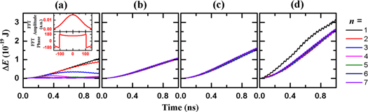
Zoom In Zoom Out Reset image size

Figure C3 displays the increase in total energy (ΔE) of the seven normal modes under temporal and multidimensional resonance conditions. The oscillation amplitude of the external field is small (10 Oe) to suppress nonlinear dynamics. To make the results comparable, we keep the summation of the magnetic flux (absolute value) in all phase zones the same in the simulations. The temporal resonance in figure C3(a) shows the highest energy growth rate at n = 1 and a much lower rate as n increases, with the exception of n = 2. The resonance frequency at n = 2 is very close to that at n = 1. As a result, the spin wave excited by a globally uniform field at frequency ν₂ resembles the fundamental mode rather than the n = 2 mode, as displayed in the inset of figure C3(a). We observe significant enhancement in growth of ΔE under multidimensional resonance for all modes except the fundamental mode, as shown in figure C3(b). The spatial distribution of the external field matches the space pattern of the corresponding normal mode, but the field amplitude is uniform in each phase zone. The fundamental mode is the only mode that has a uniform phase distribution; therefore, multidimensional resonance and temporal resonance produce the same result at n = 1. The growth rate of ΔE increases by approximately 50% for all modes when the external field aligns with not only the space pattern but also the mode amplitude profile, as shown in figure C3(c). In figure C3(d), we observe the greatest energy growth rate when the external field is concentrated at the antinodes. The rate is approximately 100% higher for n = 1 and 67% higher for n ≥ 2 than the results in figure C3(c).

Zoom In Zoom Out Reset image size