


Abstract
Phosphorene (a monolayer of black phosphorus) is a large gap semiconductor with high mobility and has great application potential. Numerical calculations reveal that phosphorene is a topologically trivial material and can only host edge bands on specified edges such as the zigzag edge. A linearly polarized irradiation on the phosphorene lattice results in the dynamic gaps in the quasi-energy spectrum. We found that the irradiation polarized in the zigzag direction induces new edge bands within the dynamic gaps on any type of edge (zigzag, armchair, or other bearded edge). We proposed a new gauge independent quantity,  , to account for the appearence of universal edge bands, where δ is the detune and g is the light induced valence-conduction band transition element. The number of edge bands in the dynamic gaps is reflected by the winding number of it.
Export citation and abstract BibTeX RIS

Original content from this work may be used under the terms of the Creative Commons Attribution 3.0 licence. Any further distribution of this work must maintain attribution to the author(s) and the title of the work, journal citation and DOI.
1. Introduction
Periodically driving can turn a normal material into the so-called Floquet topological insulator [1–5]. Light irradiation is an important periodic driving source and its impact on materials draws much attention. Recently, the Floquet topologic phase of condensed matter materials and photonic crystals were observed experimentally [6, 7], and verified the validity of the theoretical prediction and showed the potential application of irradiation for topologic phase engineering. Light irradiation affects the bulk band structure of materials by two mechanisms. First, the electron near the neutral point of gapless materials, such as graphene, emits a photon and re-absorbs it to renormalize the band structure, and so a mini-gap is generated at the neutral point [8–11], which is a second order effect. Secondly, light induces resonant transition between conduction band and valence band states, and results in dynamic gaps in the quasi-energy spectrum at  , where ℏ is the reduced Planck constant and ω is the angular frequency of light [12–15]. The latter is more attractive because it is a first order process and will be considered in this paper. If the light is circularly polarized, it can change the material's topological property, which is reflected by the arising of new helical edge bands in the dynamic gaps [14–17]. These photon-exited spectrums can be detected by the Angle-resolved photoemission spectra measurement [7]. Because the illuminated system is not an equilibrium one, the occupation rule of the quasi-energy spectrum is complicated, and the edge band induced by irradiation does not carry exactly one conductance quanta in electronic transport [18–22].
Phosphorene, a monolayer of black phosphorus, has great potential for electronic application because its field-effect transistors have a large on-off current ratio at room temperatures [23–25]. Its energy gap is moderately large and its anisotropy is quite strong. By applying static strain, phosphorene can be tuned into a band-inversion material [26, 27], which could host topological node-line states near the Fermi energy [28]. Vertical electric field can make phosphorene become a Dirac semimetal [29] and induces a topological phase transition in few-layer phosphorene [30]. The linearly polarized laser illumination results in dynamic gaps in the quasi-spectrum of phosphorene, but cannot induce topological phase transition [31]. In this paper, we investigated the band structure of phosphorene ribbons under linearly polarized irradiation. We found that in the dynamic gaps, there exist edge bands on both zigzag and armchair edges if the polarization is along the zigzag direction, but no edge band appears when the polarization is along the armchair direction. Whether or not edge bands exist in the dynamic gaps is governed by a gauge independent quantity,  , with δ being the detune and g being the light induced valence-conduction band transition element. For the polarization along other directions, the zigzag component and the armchair component of the polarization vector compete with each other. When the polarization is deviated from the zigzag direction, the k-interval of edge band existence shrinks and it vanishes for a critical polarization orientation.
2. Hamiltonian
The phosphorene lattice is composed of puckered-up and puckered-down phosphorus atoms as demonstrated in figure 1. The in-plane structure of the phosphorene is a deformed honeycomb lattice with the in-plane parameters a = 0.8014, bx = 1.515, and by = 1.674 (in units of Å) [32]. The x-axis and y-axis are set to be parallel to the armchair and zigzag directions. Because there is no difference between the on-site potentials on the puckered-up and puckered-down atoms, the phosphorene lattice can be regarded as a bipartite system consisting of A and B sublattices, as shown in the inset. The five types of nonzero hoppings are labeled by  and t0 in the figure, the values of which are 3.665, −1.220, −0.205, −0.005 and −0.105 (in units of eV), respectively [33]. The tight-binding Hamiltonian reads

where the summation runs over all nonzero hoppings. In basis of A-B sublattices, the k-space Hamiltonian is

The elements h0 and h are both of the form

where rα denotes the position vector from an A-site pointing to nearby A- or B-site, and tα is the corresponding hopping. The matrix elements are calculated as

where  and dy = by. Solving the Hamiltonian, we have the conduction band and valence band energies

and the corresponding eigen states

where  and
and  are the conduction and valence band sates respectively and ϕ is the complex angle of h. When a polarized light irradiates normally on the phosphorene sheet, the light can be described by a time-dependent vector potential
  , where
  is the amplitude vector and t is the time. The vector potential can be involved into the Hamiltonian by the Peierls substitution (Form here on, ℏ and e in equation expressions are set to be unit to simplify the derivation)

This leads to the additional time-dependent Hamiltonian

In basis of  and
and  , we apply the rotating wave approximation and have the Hamiltonian

where g is the transition element defined by

One can verify that  is a pure imaginary quantity (see the
  as
as  and we have

The time-dependent Shrödinger equation of the Hamiltonian Ht can be numerically solved in the Floquet space in basis of  with n being an integer. The quasi-spectrum can be obtained by averaging the density of states over a period of driving. In this paper, we instead use the method described in [31] to calculate the quasi-spectrum of phosphorene ribbons. The studied armchair and zigzag ribbons lie along x and y directions, respectively, according to the axis definition in figure 1.

Figure 1. Sketch of phosphorene lattice, in which red- and blue-filled circles represent puckered-up and puckered-down phosphorus atoms respectively. The inset shows the bipartite strucuture of the phosphorene lattice consisting of A and B sublattices.
Download figure:
Standard image High-resolution imageFigures 2(a)–(d) show the quasi-spectrum for phosphorene ribbons under the irradiation polarized along x- and y-directions3 . In the band gap of the zigzag ribbon, the nearly flat edge bands survive but are disturbed a little by the irradiation, which is not our target in this paper. (The origination of the edge bands of un-irradiated phosphorene ribbons was discussed in [34] and [35], which can be explained by the winding number analysis of h by choosing proper gauges for the armchair and zigzag edges respectively. The winding number reflects the number of edge bands and was proven to be 0 for armchair ribbons and 1 for zigzag ribbons). Within the conduction or valence band, the irradiation induces the so-called dynamic gap. Interestingly, one can find that new edge bands appear in the dynamic gaps if the polarization is along y-direction (the zigzag direction) regardless of the edge type of the ribbons. This means there must be a new gauge invariance to govern the existence of those edge bands, which will be explored in the following.

Figure 2. (a–d) Quasi-energy band strucuture of Ht, (e–h) band structure of  , (i–l) components of
  at resonance as functions of wavevector, and (m–p) winding number pictures of η for the wavevectors labeled by the bold dots. Both the armchair and zigzag phosphorene ribbons have 200 transversal atoms. The ribbons are irradiated by linearly polarized light with the frequency
  eV and with polarization amplitude Ax = 0.1 for x-polarization and Ay = 0.1 for y-polarization (the in-plane parameter a is treated as the unit length). The vertical dashed lines indicate the the intervals for vy0, also the intervals for edge band existence.
Download figure:
Standard image High-resolution image3. Spectrum and edge bands
To find out the physics within the dynamic gaps, we use the time-dependent unitary transformation

where  is the detune, to reduce the time-dependent Hamiltonian Ht into a static one, saying

By means of the unitary matrix

we transform the reduced Hamiltonian  into
into

with

The eigen values of the effective Hamiltonian  are
are  . Because
  is deduced from the original time-dependent Hamiltonian Ht without approximation, all the information of the irradiated system is encoded in the effective Hamiltonian. Figures 2(e)–(h) show the dispersion of
  for the irradiated phosphorene ribbons with zigzag and armchair edges. The features of the quasi-energy bands of Ht can be found their reflection in the band structure of
  : the two dynamic gaps for Ht merge in the spectrum of
  and so do the edge bands.
The winding number of the effective Hamiltonian can be used to handle the edge bands of the ribbons. The complex quantity η has the real part δ and the imaginary part  . For a ribbon lying along x direction (armchair ribbon), kx is a good quantum number. At a given quantum number kx, η is a function of parameter ky. When the parameter ky changes though out the Brillouin zone, the endpoint of the complex vector of η on the complex plane moves and evolves as a closed curve. The turn of times of the curve around the origin is called the winding number. Similarly, if the ribbon lies in y-direction (zigzag ribbon), ky is a good quantum number, and trajectory of the endpoint of η is a closed curve when the parameter kx changes through out Brillouin zone. To reflect the number of edge bands, the winding number analysis should use different gauges for different types of edge. We consider the gauge transformation Ug, which transforms the operator
  to
to  and translates the state
  (
( ) to
) to  . According to equation (10), g keeps unchanged under the gauge transformation, and so η is a gauge invariable. This means that the existence of edge bands in the dynamic gaps is independent of the edge type.
Firstly we consider the irradiation is polarized in x-direction (the armchair direction). For this case we have  (Ax is set to be a unit which has no influence on the winding number analysis). The trajectory of the endpoint of η for the armchair ribbon at the wavevector denoted by the bold dot in figure 2(e) is shown in figure 2(m). Because vx is even with respect to kx and ky (see the
  . Because the trajectory curve modifies when the wavevector (kx or ky, depending on the ribbon orientation) varies, the resonant value of vx is a function of kx (or ky) [31]. We define the resonant response quantities

to understand the property of dynamic gap. Figures 2(i) and (k) show the function of vx0 versus kx for the armchair ribbon and that versus ky for the zigzag ribbon, respectively. One can see that consistency between the curve shape and the profile of the dynamic gap in the spectrum.
Secondly, we assume that the irradiation polarization is in the y-direction (the zigzag direction), and we have  (Ay is set to be a unit). Figures 2(n) and (p) show the winding number pictures at the wavevectors represented respectively by the bold dots in figures 2(f) and (h). The trajectories of η are up-down symmetric closed curves, because vy is a odd function of kx and ky (see the
We also check the spectrum of the effective Hamiltonian for phosphorene ribbons with other edges (not shown), such as bearded zigzag and bearded armchair, under linearly polarized illumination, and verify our conclusion: if the polarization is along the zigzag direction, edge bands arise in the dynamic gap, and if along the armchair direction, no edge band turns up.
When the polarization is along neither x- nor y-direction, we have  . The complex number η can be decomposed to
  and
and  . The trajectory of the former for the armchair or zigzag ribbon is just the curve in figure 2(n) or (p) amplified along the imaginary axis by the factor Ay. The distance between the intersect points on the imaginary axis is
  . If we pick the latter part up, it lift the amplified curve vertically by the amount
  , but the intersect point distance
  is not affected by the lift. Figures 3(e) and (f) show the trajectory of η for armchair and zigzag ribbons at the wavevectors denoted by the bold dots. The shape of the trajectory curve of η is deformed and asymmetric, because the lift amount
  is not a constant when the wavevector varies. In figure 3(e), the lift amount is large enough so that the origin is exposed outside out the trajectory curve. Therefore, there is no edge state at the selected wavevector. For the case of figure 3(f), the lift amount is not such large, the origin is included by the trajectory, and one can find the edge band states in the spectrum at the corresponding wavevector.
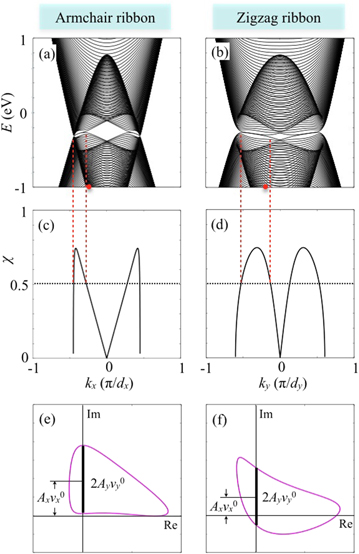
Figure 3. (a, b) Band structure of  , (c, d) χ as function of wavevector, and (e, f) winding number pictures for the wavevectors labeled by the bold dots. The phosphorene ribbons have 200 transversal atoms and the irradiation parameters are
  eV, Ax = 0.05, Ay = 0.1, and
  . The vertical dashed lines indicate the the intervals for
  , also the intervals for edge band existence.
Download figure:
Standard image High-resolution imageThe inclusion of the origin is determined by the competition between  and
and  . If
. If  , the origin is inclosed in the trajectory curve and the winding number is 1. We define the ratio
  as an intrinsic quantity to characterize the response to the polarization and the ratio
  to indicate the polarization orientation, and we have condition for edge state appearing as

Figures 3(c) and (d) show the curves of χ versus the wavevector. For a given polarization orientation, one can find the interval for edge states appearing by cutting the curves of χ with the horizontal line  as shown in the figures. The vertical dashed lines is used to illustrate the interval of the edge bands surviving. Now we consider the polarization is initialized along y-direction (Ax = 0), and then turn on x-component and increase it. The line of
  moves up, the interval of edge bands will shrink and finally disappear when the horizontal line reaches the maximum of the χ curve. If the polarization is more deviated from y-direction, the horizontal line cannot cross the curve of χ, and the upper and lower bands depart away from each other completely.
4. Conclusion
Linearly polarized irradiation induces edge bands in phosphorene ribbons on any type of edge in the dynamic gaps if the polarization is along the zigzag direction. The appearing of the universal edge bands is determined by the winding number of  . It is gauge independent, and thus is unrelated with the edge type.
Acknowledgments
This work was supported by the National Natural Science Foundation of China Grants No. 11274124 and No. 11474106, and No. 11575051.
: Appendix. Symmetry of 

The winding number of η has tight relation with the symmetry of  . According to the amiltonian in equation (2) and the eigen states in equation (6), the quantity
  is calculated as


It is pure imaginary, and we have the expression of  ,
,

Its symmetry relies on the properties of h and  . The expression of h in equation (4) ensures the following relations

and correspondingly, we have

Now we consider the symmetry of the x component of  ,
,

We proved that vx is even about kx and ky. Turn to the y component, we have

So we verified that vy is an odd function of kx and ky.
Footnotes
- 3
The quasi-spectrum is composed by weighted quasi-energy band dispersions. The dispersion weight is often indicated by the transparency of the dispersion curves [14, 31]. To avoid the obscure of the curves with different transparency and to make the figures more clear, the quasi-energy dispersions with the weight greater than 0.4 are plotted in solid lines, and those with the weight less than that value are invisible in this paper.