


Abstract
From a physics point of view, the emergence of a traffic jam is considered to be a dynamical phase transition. To verify this, we performed a series of circuit experiments. In previous work, Tadaki et al (2013 New J. Phys 15 103034), we confirmed the occurrence of this phase transition and estimated the critical density between free and jammed flows by analyzing the fundamental diagram. In this paper, we characterize and distinguish free and jammed flows, beyond the analyses of fundamental diagrams, according to the distribution and correlation of experimental speed data. We find that the speed in free flow does not correlate and its distribution has a narrow single peak at the average. The distribution of speed in jammed flow has two peaks or a single broad peak. The two peaks indicate the car speeds inside and outside of jam clusters. The broad single peak appears as a result of the appearance and disappearance of jam clusters. We also find that the formation of jam clusters induces a long correlation in speed. We can identify the size of jam clusters and the relative distance between coexisting jam clusters from this speed correlation.
Export citation and abstract BibTeX RIS

Original content from this work may be used under the terms of the Creative Commons Attribution 3.0 licence. Any further distribution of this work must maintain attribution to the author(s) and the title of the work, journal citation and DOI.
1. Introduction
Traffic jams are a familiar phenomenon on expressways and city streets. We empirically recognize that there are two types of traffic flows: flows with slow or stopped cars (jammed or congested flows) and smooth flows. Since the 1990s, traffic flows have attracted research interests from a physics point of view [1–7]. Various theoretical models of traffic flow have been proposed and studied. Flow on a circuit has been studied as the most fundamental cases. These researches have clarified that a homogeneous flow becomes unstable and forms traffic jam, when the density of cars exceeds a critical value. In this sense, the emergence of traffic jams is understood as a dynamical phase transition, in which the car density is the control parameter.
Traffic data taken from expressways have been compared with theoretical studies. One conventional method for studying such traffic data involves examining a fundamental diagram representing the relation between traffic density and flow. Theoretical studies have succeeded in reproducing the observed features of these fundamental diagrams [8–11]. However, fundamental diagrams provide limited information about a flow, because the observed quantities used in fundamental diagrams are time averages at an observation point. In other words, the spatial structure of the flow is not considered. Moreover, fundamental diagrams do not capture all characteristics of jam clusters, because stopped cars do not contribute to fundamental diagrams [9, 12].
Experimental studies of traffic flow enable a deeper understanding of the properties of traffic flow. For this purpose, we conducted two circuit experiments. In the first experiment, a circuit was placed in an outdoor environment, and we confirmed the emergence of a traffic jam without a bottleneck [13, 14]. A homogeneous flow was observed before the emergence of the traffic jam. As a result, we experimentally confirmed that high-density homogeneous flow becomes unstable and a traffic jam emerges.
The second experiment was performed on an indoor circuit set in Nagoya Dome. We experimented with various number of cars. In our previous paper [12], all flows were classified as one of four types based on the fundamental diagram: free flow, jammed flow, stop-and-go flow and other flows with densities between those for free and jammed flows. When the car density was low, jam clusters did not appear, and free flow was realized. This free flow is characterized as a low-density and high-speed smooth flow. When the car density was high, the jammed flow or stop-and-go flow was realized. The jammed flow is characterized by the existence of jam clusters in which cars move slowly. The stop-and-go flow is distinguished from the jammed flow by the presence of stopped cars inside the jam clusters. At intermediate densities, both free and the jammed flows were observed. We estimated the critical density that separated the free flows from the jammed flows. The estimated critical density is compatible with the value for real expressways. Based on the experimental data, we study the scaling relation of the critical density in a separate paper [15] 8 .
In this paper, by inspecting the data obtained from the second experiment, we examine the properties of flows beyond the analyses of fundamental diagrams. Our aim is to identify the physical quantities that characterize traffic flows. The formation of jam clusters divides cars into two broad groups: slow cars inside the jam clusters and fast cars outside. As a result, the existence of jam clusters induces changes in the distribution and correlation of traffic speed. Thus, the distribution and correlation of speed are the physical quantities that characterize free and jammed flows. We also investigate the dynamical change in the distribution and correlation according to the appearance and disappearance of jam clusters in jammed flows.
This paper is organized as follows: section 2 briefly describes the outline of the second experiment and the measured data. In section 3, the distribution and correlation of speed are studied for free, jammed and stop-and-go flows. In the case where jam clusters appear and disappear, we also examine the time evolution of the distribution and correlation of speed. Time evolutions of flows at intermediate densities are studied in section 4. The positions of the two peaks in the speed distribution are discussed in section 5. Section 6 is devoted to summary.
2. Outline of the experiment and the data
The experiment was performed on an indoor circuit of 100 m diameter within Nagoya Dome. We conducted 19 sessions with 10–40 cars over a period of two days. Each session was given a 4-digit identification number: the first two digits are the serial number and the last two digits denote the number of cars in the session. In this paper, because we study properties of flows according to the types shown in the previous paper, we select data from 14 sessions (table 1) consisting of four warm-up sessions on the first day and 10 sessions on the second day. The remaining 5 sessions on the first day are discussed in appendix
Table 1. List of session IDs and the numbers of cars for 14 sessions. The last two digits of the session ID expresses the number of cars N in the session. The periods used in the analyses were set by discarding the beginning and end of each session.
| Session ID | N(# of cars) | Total running time (s) | Period used in analyses (s) | ||
|---|---|---|---|---|---|
| 1010 | 10 | 431 | 150 | – | 400 |
| 1210 | 10 | 380 | 0 | – | 250 |
| 1310 | 10 | 413 | 50 | – | 300 |
| 1412 | 12 | 465 | 100 | – | 350 |
| 2030 | 30 | 817 | 100 | – | 700 |
| 2125 | 25 | 622 | 100 | – | 500 |
| 2228 | 28 | 636 | 100 | – | 450 |
| 2328 | 28 | 498 | 100 | – | 350 |
| 2432 | 32 | 824 | 100 | – | 700 |
| 2534 | 34 | 769 | 100 | – | 600 |
| 2634 | 34 | 902 | 150 | – | 700 |
| 2732 | 32 | 747 | 150 | – | 700 |
| 2830 | 30 | 743 | 100 | – | 600 |
| 2934 | 34 | 421 | 100 | – | 300 |
A laser scanner was located at the center of the circuit to record the positions of the cars. The data were used to construct sequences of the headway and car speeds. The acquired data had a temporal resolution 0.2 s and a spatial resolution 0.16 m. Appendix
3. Characterizing three types of flows using the distribution and correlation of speed
3.1. Distribution and correlation of speed
Speed and headway are fundamental quantities for microscopic description of traffic flows. As shown in the following, we can obtain clearer features by analyzing the distribution and correlation of speed than those of headway. The distribution and correlation of headway are discussed in appendix
Figure 1 shows the evolutions of car speed from typical sessions showing three flow types: free, jammed and stop-and-go flows. Free flow (session 2125, figure 1(a)) allows cars to run smoothly with sufficiently large headways. As a result, the speed of each car fluctuates independently around the average ( ). In stop-and-go flow (session 2030, figure 1(c)), the speed of each car exhibits large amplitude oscillations, reflecting the car speed inside and outside of the jam cluster, in which cars are forced to stop. The jam cluster propagates backward against the motion of cars (toward the smaller car indexes in figure 1). Figure 1(b) shows the evolution of car speed in the jammed flow (session 2634). The speed of each car oscillates considerably, but does not decrease to zero. In this flow type, jam clusters appear and disappear. Other flows at the intermediate density are analyzed in section 4.
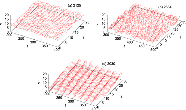
Figure 1. Typical evolution of speed for each car for (a) free, (b) jammed, and (c) stop-and-go flows. The vertical (v) and horizontal (t) axes denote speed and time respectively. The depth (i) axis denotes car indexes.
Download figure:
Standard image High-resolution imageFirst we study the speed distributions with the aim of characterizing the flows. The speed distribution for each session is obtained by accumulating the car speed during the period defined in table 1. In free flow, the car speed fluctuates around the average, as shown in figure 2(a). The speed distribution for stop-and-go flows has two peaks, representing the car speeds inside and outside of jam clusters (figure 2(c)). Hereafter, we refer to the peak in the high-speed region as the mode speed vM. In jammed flows, the speed is broadly distributed around the mode speed vM (figure 2(b)).

Figure 2. Speed distribution for (a) free, (b) jammed, and (c) stop-and-go flows. The bin size is 0.4 m/s.
Download figure:
Standard image High-resolution imageNext, we focus on the speed correlation for each flow type. The correlation in speed is defined as


where  denotes the speed of the ith car at time t, and the summation runs over all car indexes i and all time slices t (every 0.2 s) in the period defined in table 1.
Figure 3 shows the scaled speed distributions (upper row) and the corresponding correlation (lower row). We employ scaled horizontal variables for studying characteristic features for three types of flows. The speed distributions for free flows are shown against the speed scaled by the average speed in that session, and those for jammed and stop-and-go flows are shown against the speed scaled by the mode speed vM in that session. The horizontal axis ξ for the speed correlation is the car-index spacing (j in equation (1)) divided by the total number of cars in the session.

Figure 3. Distribution (upper) and correlations (lower) of speed for all sessions. The horizontal axes for the speed distribution are normalized with the average speed for free flows (a) and with the mode speed for jammed (b) and stop-and-go flows (c). The horizontal axes for the speed correlations ((a*), (b*), and (c*)) give the relative car index divided by the total number of cars in the session.
Download figure:
Standard image High-resolution imageIn free flows, the speed distributions are almost the same as the normal distribution of the same width centered around the average speed (figure 3(a) and detailed features are given in appendix  , which corresponds to one or two car-index spacings. In other words, the speed is not correlated9
.
, which corresponds to one or two car-index spacings. In other words, the speed is not correlated9
.
In stop-and-go flows, the speed distribution has two peaks representing the speed of cars inside and outside of jam clusters (figure 3(c)). A detailed analysis of the speed distribution in these cases is given in section 5. The existence of jam clusters induces a long speed correlation (figure 3(c*)), where the correlation extends to the system size (i.e., the number of cars in the session). The upward-convex shape of the correlation around  indicates the existence of a long-range correlation. The negative correlation around
  means that, for a car within a jam cluster, the car at the opposite side of the circuit is running outside of the jam cluster, and vice versa. The value ξ at which the correlation becomes zero corresponds to the number of cars in the jam cluster.
In jammed flows, the speeds are broadly distributed as a result of the formation of jam clusters (figure 3(b)). The existence of jam clusters again induces long correlations in speed (figure 3(b*)). A detailed analysis for this case is given in section 3.2.
3.2. Appearance and disappearance of jam clusters in jammed flows
We now study the properties of the jammed flow in session 2634 as an example. Figure 4 shows the spacetime diagram of car trajectories, with different colors denoting different car speeds. Jam clusters (blue regions) propagate backward against the motions of the cars, and temporarily disappear. The initial jam cluster starts to dissolve around 220 s, and the flow becomes almost smooth, albeit with fluctuations, until 550 s. During this period, the jam clusters appear and disappear. Moreover, more than one jam cluster can sometimes coexist. During the period 550–650 s, a jam cluster distinctly emerges.

Figure 4. Spacetime diagram for session 2634, where cars run from left to right. The colors of the data points represent the speed of the cars.
Download figure:
Standard image High-resolution imageTo investigate the time evolution of the distribution and correlation of speed, we calculate the averages over 60 s windows. Figure 5 shows the distribution and correlation of speed in four typical periods. During the period in which the initial jam cluster exists, (200–250 s), the speed was broadly distributed (figure 5(a)) and the flow exhibits a long correlation (figure 5(a*)). After the initial jam cluster dissolves, the speed correlation in the period 250–310 s (figure 5(b*)) has a shoulder around  , which indicates that two jam clusters coexist approximately seven cars apart, as seen in the spacetime diagram (figure 4). For the period 350–410 s (figure 5(c)), the distribution has a single peak. At first glance, this seems to indicate free flow, but the width of the peak is too broad. The correlation has another lower peak at around
  (figure 5(c*)), which indicates the coexistence of two jam clusters at opposite sides of the circuit. In this case, the car speeds are not particularly slow in these jam clusters. Hereafter, we call these weak jam clusters. These weak jam clusters are not clearly visible in the spacetime diagram. In the last period (550–610 s), the distribution (figure 5(d)) and the correlation (figure 5(d*)) are similar to those observed in the stop-and-go flows (figures 3(c) and (c*)). This shows that a jam cluster distinctly exists. The full temporal evolution of the distribution and correlation are shown in appendix

Figure 5. Snapshots of the evolution of the distribution (upper row) and correlations (lower row) of speed in session 2634. The distributions and correlations are evaluated as a 60 s moving average. Arrows denote characteristic features indicating the coexistence of jam clusters.
Download figure:
Standard image High-resolution imageBy studying the average distribution and correlation over 60 s windows, we can observe the appearance and disappearance of jam clusters. The analysis of the correlation enables us to estimate the number of cars in the jam cluster and the distance between two coexisting jam clusters. Moreover, this analysis allows us to identify weak jam clusters, which are not always visible in the spacetime diagrams.
4. Applications to flows at intermediate densities
In our previous paper, three sessions (2228, 2328 and 2830) with densities between the free flows and jammed flows were not classified clearly by the analysis of the fundamental diagrams. Here, we apply the analysis proposed in section 3.2 to characterize the flows observed in those sessions. The relevant spacetime diagrams are shown in figure 6.

Figure 6. Spacetime diagrams of flows at intermediate densities between free and jammed flow. Colors of dots denote car speeds.
Download figure:
Standard image High-resolution imageFirst, we study the time evolution of the distribution and correlation of session 2228 in figure 7. From the evolution of the speed distribution, we find that the initial jam cluster starts to dissolve (figures 7(a) to (c)) and finally a new jam cluster emerges (figure 7(d)). In the period 320–380 s, the distribution has a single broad peak, as shown in figure 7(c). However, the correlation (figure 7(c*)), which has three peaks, indicates that a few weak jam clusters coexist. In the final stage, the correlation (figure 7(d*)) shows the coexistence of a large jam cluster and a small weak one at the opposite side of the circuit.
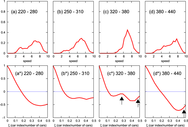
Figure 7. Snapshots of time evolution of the distribution (upper row) and correlations (lower row) of speed in session 2228. The distributions and correlations are evaluated as 60 s moving averages. Arrows denote characteristic features indicating the coexistence of jam clusters.
Download figure:
Standard image High-resolution imageIn the spacetime diagram for session 2328 (figure 6(b)), the flow appears to be free. The speed distribution in figures 8(a)–(d) exhibits a single peak. From the period 150–210 s, a jam cluster starts to emerge, but does not fully evolve. In particular, figures 8(c) and (d) exhibits sharp single peaks. However, the correlation of speed (figures 8(c*) and (d*)) indicates the coexistence of very weak jam clusters.

Figure 8. Snapshots of time evolution of the distribution (upper row) and correlations (lower row) of speed in session 2328. The distributions and correlations are evaluated as 60 s moving averages. Arrows denote characteristic features indicating the coexistence of jam clusters.
Download figure:
Standard image High-resolution imageIn session 2830, the initial jam cluster can be observed (figures 9(a) and (a*)). After this initial cluster has dissolved, a few weak jam clusters coexist (figures 9(b) and (b*)). In the period 440–500 s, a narrow single peak in the speed distribution and a short correlation length (figures 9(c) and (c*)) indicate the emergence of free flow. Toward the end of the session, a new jam cluster starts to emerge (figures 9(d) and (d*)).
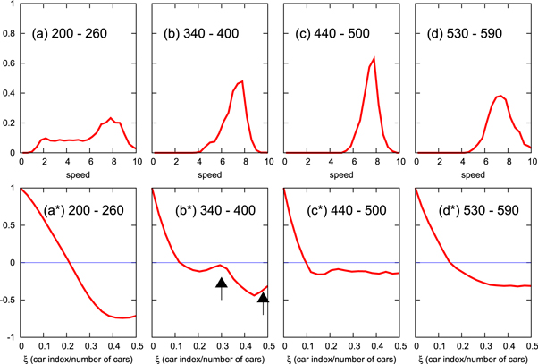
Figure 9. Snapshots of time evolution of the distribution (upper row) and correlations (lower row) of speed in session 2830. The distributions and correlations are evaluated as 60 s moving averages. Arrows denote characteristic features indicating the coexistence of jam clusters.
Download figure:
Standard image High-resolution image5. Speed distribution for flows with jam clusters
In this section, we study the speed distribution of flows, in which jam clusters distinctly exist. We begin by examining stop-and-go flows (sessions 2030 and 2934). In session 2934, the slowest speed was zero except for a short initial period at the start of the session. In other words, the jam cluster in session 2934 always contained some cars stopped completely. In session 2030, however, the jam cluster consisted of slow-moving cars in some periods and stopped cars in other periods. To examine the differences in jam clusters with and without stopped cars, we analyze the distributions averaged over 60 s windows. The speed distribution in the period with stopped cars (430–460 s for session 2030 and 200–300 s for session 2934) is shown in figure 10(a), and that for the period without stopped cars (200–400 s for session 2030) is presented in figure 10(b).
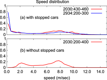
Figure 10. Speed distribution for periods with and without stopped cars.
Download figure:
Standard image High-resolution imageThe speed distributions for periods with completely stopped cars have two peaks (figure 10(a)), with the slower peak located at zero. In contrast, the speed distributions for the period without completely stopped cars have two peaks, the slower peak of which is located at a non-zero speed (of approximately 2 m/s) (figure 10(b)). The faster peak is located at a slightly slower speed than that for the flow with stopped cars. This suggests there is the relation between the locations of faster and slower peaks: when the slower peak is located at a higher speed, the faster peak will be at a slower speed.
Another example can be found in jammed traffic flow. In session 2634, a jam cluster emerged in the period 550–610 s, the speed distribution of which has two peaks (figure 5(d)). It can be seen that the slower peak is located at a higher speed (about 2.5 m/s) than in figure 10(b), whereas the faster peak is located at lower speed (6 m/s). The difference between the two peaks is smaller than in the case shown in figure 10(b).
This can be roughly explained as follows. The faster a car is driving, the longer time it needs to decelerate while slowing down when joining a jam cluster. As a result, the headway in the jam cluster becomes shorter, and the speed in the jam cluster is slower. This is discussed more precisely in appendix
6. Summary
We have studied the characteristic features of free and jammed flows based on experimental data [12]. For this purpose, we investigated the distribution and correlation of speed. In free flows, the average headway is sufficiently large and the speeds fluctuate randomly around the average. The car speeds are not correlated, and are narrowly distributed about the average. Once the car density exceeds a critical value, jam clusters emerge. As a result, the speed distribution exhibits two peaks corresponding to the car speeds inside and outside of these jam clusters. Speed distributions with two peaks have also been reported in observations of highway traffic [11]. The existence of jam clusters induces a strong correlation in speeds, which agrees with observational data [9].
In jammed flows, jam clusters appear and disappear, and multiple clusters sometimes coexist. Our analysis of the distribution and correlation of speed enables the emergence of weak jam clusters and their coexistence to be identified, even if the flow appears to be smooth in spacetime diagrams. Moreover we can determine the size of jam clusters and the relative distance between jam clusters from the speed correlation. In summary, the distribution and correlation of speed are keys factors in distinguishing the existence of jam clusters and analyzing their properties.
Acknowledgments
We thank Nagoya Dome Ltd., where the experiment was performed. We also thank SICK K K for their technical supports on the laser scanner. We thank H Oikawa and students from Nakanihon Automotive College for assisting with the experiment. This work was partly supported by the Mitsubishi Foundation and JSPS KAKENHI Grant Number 20360045.
Appendix A.: Time evolution of the distribution and correlation of speed in session 2634
In the main text, snapshots selected from the time evolution of the distribution and correlation of speed in session 2634 were presented to describe the appearance and disappearance of jam clusters. This appendix shows their full time evolution. Each curve is evaluated over 60 s windows.
As shown in figure 4, the session initially contained a jam cluster, but this disappeared around 350 s (figure A1). The flow then became almost homogeneous in speed. However, the speed distribution is broad and the correlation indicates the coexistence of jam clusters (figure A2).
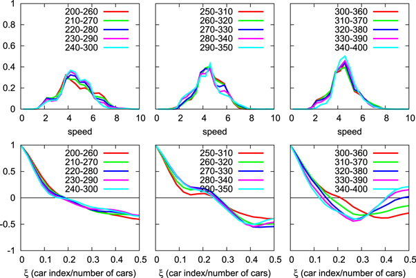
Figure A1. Time evolution of the distribution and correlation of speed in session 2634 from 200 s to 400 s.
Download figure:
Standard image High-resolution image
Figure A2. Time evolution of the distribution and correlation of speed in session 2634 from 350 s to 550 s.
Download figure:
Standard image High-resolution imageAfter the period mentioned above, a jam cluster distinctly emerged at around 550 s. Two peaks emerged in the distribution of speed, reflecting the speed of cars inside and outside of the jam cluster. The length of the correlation increased, and began to resemble that for stop-and-go flows (middle of figure A3). This jam cluster then started to disappear (bottom of figure A3), causing the speed distribution to become narrower and the correlation length to decrease.
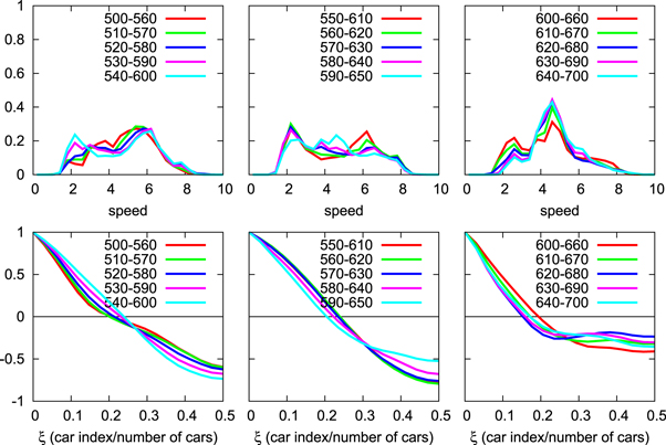
Figure A3. Time evolution of the distribution and correlation of speed in session 2634 from 500 s to 700 s.
Download figure:
Standard image High-resolution imageAppendix B.: Distribution and correlation of headway
The formation of jam clusters would be also determined by changes in the distribution and correlation of headway. In free flows, drivers are allowed to maintain their preferred headway to the preceding car, and large amplitude fluctuations in headway are permissible. Thus, the distribution of headway for free flows has irregular features as shown in figure B1 (a), representing driver's various preferences. As a result, the headway does not exhibit any correlation (figure B1(e)).
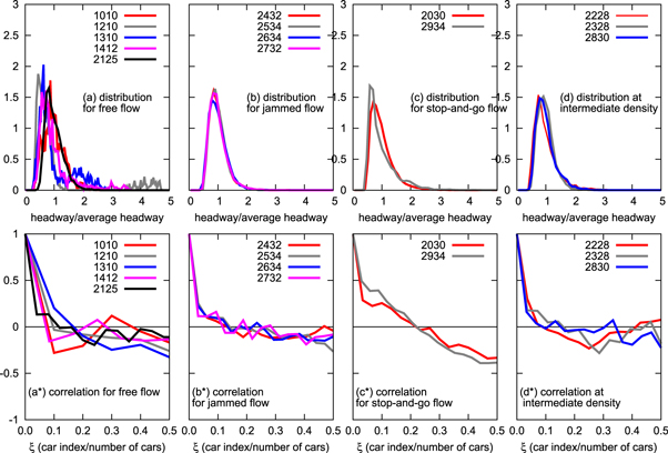
Figure B1. Headway distribution and correlations for all sessions. The horizontal axes for the correlations are the relative car index divided by the total number of cars in the session. The horizontal axes for the distribution are normalized with the average headway.
Download figure:
Standard image High-resolution imageBoth in jammed and stop-and-go flows, the headway distribution has a single peak (figures B1(b) and (c)). Because the headway of cars cannot vary significantly in these flows, the irregularity observed in the distribution for free flows is reduced. In spite of the formation of jam clusters in these flows, the distribution has a single peak. This is because a narrow range of headway is available and headway values for car motion outside of jam clusters are broadly distributed (figure B2). Thus, the peaks for headways inside and outside of jam clusters overlap, and a single peak is observed.

Figure B2. Speed and headway distribution for session 2030. In headway-speed plain, two peaks for inside and outside of jam clusters locate separately. In the projection to speed axis, these two peaks are clearly separated. However, in the projection to headway axis, they are closely overlapped.
Download figure:
Standard image High-resolution imageDifferent features of the headway correlation can be found in jammed and stop-and-go flows. In jammed flows, jam clusters do not propagate stationary, and when the jam cluster disappear, drivers maintain their preferred headway. Thus, the correlations in headway become shorter. In stop-and-go flows, however, cars are forced to maintain headways inside and outside of the jam clusters. As a result, the headways correlate strongly in stop-and-go flows.
Flows at the intermediate density consist of two types of flows. A smooth flow was realized in session 2328. However, the distribution of headway differs from that of free flows, because the density is too high enough allowing cars to maintain their preferred headway. Thus, the distribution of headway for these three flows exhibit the same characteristics as for jammed flows.
In summary, the existence of jam clusters does not change the distribution of headway distinctly. However, the correlation length of the headway increases if the flow contains jam clusters.
Appendix C.: Speed distribution in optimal velocity model
In the optimal velocity (OV) model [16, 17], traffic jams are characterized as a hysteresis-loop trajectory in the headway-speed plane. The higher the speed of flow outside the jam cluster, the slower the car speed within the jam cluster is. Thus, the formation of a jam cluster with (almost) stopped cars appears as a pair with the high-speed flow outside the jam cluster. If the speed of the flow outside the jam is not sufficiently high with some reasons, the speed within the jam clusters would not be slow. This is compatible with the results of our experiment.
The emergence of jam clusters with slow-moving cars can be observed in a simulation based on the OV model. If all parameters relating to a car are the same, stop-and-go flow emerges for certain sets of parameters. However, if the maximum speed distributes around the average value, the average speed outside of jam clusters decreases, because the existence of cars running a little slowly outside of jam clusters. As a result, cars do not stop and run slowly in jam clusters as shown in figure C1.

Figure C1. Speed distribution in simulations with the OV model. The speed distribution with uniform car specifications is shown in red. The speed distribution with cars with various maximum speed is shown in green. Distributed maximum speed decreases the speed outside of jam clusters, and thus increases the speed in jam clusters.
Download figure:
Standard image High-resolution imageThe emergence of jam clusters with slowly moving cars has also been discussed in terms of the characteristics of flows upstream [18]. At a bottleneck, the speed may be reduced to some value vR, which is slower than the maximum value outside the bottleneck. Upstream of the bottleneck, a flow speed of vR is realized. At an intermediate distance from the bottleneck, the flow oscillates and contains jam clusters with slowly moving cars. At a distance, finally, the flow exhibits stop-and-go motion. From these studies, it is apparent that a reduction in speed outside of jam clusters induces slow-moving cars in jam clusters.
Appendix D.: Detailed speed distribution for free flows
Figure D1 shows the detailed features of the speed distribution with the normal distribution

with  and
and  , and the Laplace distribution

with  . We can see that the speed distributions for free flows are almost the same as the normal distribution except session 1210.

Figure D1. Detailed speed distribution for free flows. The distributions are compared with normal  and Laplace
  distributions.
Download figure:
Standard image High-resolution imageAppendix E.: Analyses of 5 sessions on the first day
In the main text, we analyze 14 sessions selected 19 session as in the previous paper [12]. As pointed in the previous paper, 5 remaining sessions showed different properties from selected 14 sessions, because drivers might be extremely cautious on the first day. In this appendix, the distribution and correlation of speed for those 5 sessions are shown in figure E1.
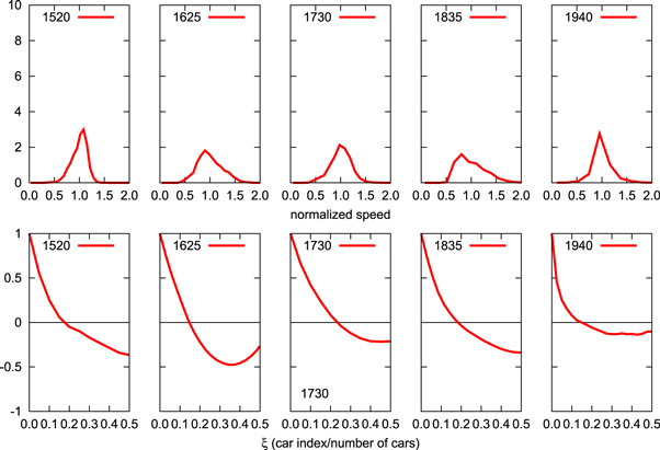
Figure E1. Distribution (upper) and correlations (lower) of speed for 5 sessions on the first day. The horizontal axes for the correlation gives the relative car index divided by the total number of cars in the session.
Download figure:
Standard image High-resolution imageAll sessions except 1940 shows typical features of jammed flow: the distribution is wide and the correlation is long but shorter than stop-and-go flows. The correlation for session 1625 indicates the coexistence of two jam clusters.
For session 1940, we find that the speed correlation is short like that in free flow. However, the distribution is wider  than that of free flow. In other word, the flow was smooth but different from low-density free flows.
Table E1. List of session IDs and the numbers of cars for 5 sessions on the first day. The last two digits of the session ID expresses the number of cars N in the session. The periods used in the analyses were set by discarding the beginning and end of each session.
| Session ID | N(# of cars) | Total running time (s) | Period used in analyses (s) | ||
|---|---|---|---|---|---|
| 1520 | 20 | 743 | 100 | – | 600 |
| 1625 | 25 | 892 | 350 | – | 750 |
| 1730 | 30 | 995 | 200 | – | 800 |
| 1835 | 35 | 1280 | 200 | – | 1000 |
| 1940 | 40 | 979 | 300 | – | 900 |
Footnotes
- 8
The raw data will be available from our web site http://traffic.phys.cs.is.nagoya-u.ac.jp/.
- 9
In figure 3(a*), the correlation in session 2125 slightly increases near
 . This may indicate that the flow is almost free but close to the transition.
