


Abstract
We study, both theoretically and experimentally, the dynamical polarizability  of
of  molecules in the rovibrational ground state of
  . Taking all relevant excited molecular bound states into account, we compute the complex-valued polarizability
  for wave numbers up to 20 000
  . Our calculations are compared to experimental results at
  (
( ) as well as at
  (
( ). Here, we discuss the measurements at
  . The ultracold Rb2 molecules are trapped in the lowest Bloch band of a 3D optical lattice. Their polarizability is determined by lattice modulation spectroscopy which measures the potential depth for a given light intensity. Moreover, we investigate the decay of molecules in the optical lattice, where lifetimes of more than
  are observed. In addition, the dynamical polarizability for the
  state is calculated. We provide simple analytical expressions that reproduce the numerical results for
  for all vibrational levels of
  as well as
  . Precise knowledge of the molecular polarizability is essential for designing experiments with ultracold molecules as lifetimes and lattice depths are key parameters. Specifically the wavelength at
  is of interest, since here, ultrastable high power lasers are available.
Export citation and abstract BibTeX RIS

Content from this work may be used under the terms of the Creative Commons Attribution 3.0 licence. Any further distribution of this work must maintain attribution to the author(s) and the title of the work, journal citation and DOI.
1. Introduction
Owing to the extraordinary control over the internal and external degrees of freedom, ultracold molecules trapped in an optical lattice represent a system with many prospects for studies in ultracold physics and chemistry [1, 2], the realization of molecular condensates [3], precision measurements of fundamental constants [4–7] and quantum computation [8, 9] and simulation [10]. In the recent years, several groups have realized the preparation of optically trapped vibrational ground state (v = 0) molecules in either the lowest lying singlet or triplet potential [11–15]. Experiments with these molecules, e.g. ultracold collisions, are typically carried out in optical lattices or optical dipole traps [16–17]. In these environments, precise knowledge of the dynamical polarizability of molecules is important for well controlled experiments.
The Rb2 molecule is one of the few ultracold molecular species currently available, with which benchmark experiments for nonpolar molecules can be carried out. Here, we investigate the dynamical polarizability  of a
of a  triplet molecule in the lowest rovibrational level of
  . A similar analysis for
  regarding the electronic ground state
  was previously carried out by Vexiau et al [18]. In addition to calculations of the frequency dependent dynamical polarizability
  , we present measurements of the real part
  at a wavelength of
  nm. The experiments are performed with molecules trapped in the lowest Bloch band of a cubic 3D optical lattice which consists of three standing light waves with polarizations orthogonal to each other. By carrying out modulation spectroscopy on one of the standing light waves, we map out the energy band-structure for various light intensities. From these measurements
  is determined. Our experimental findings at
  nm and also those at 830.4 nm [13] agree well with the calculations. In addition, we experimentally investigate the decay time of the deeply bound molecules in a 3D optical lattice at 1064.5 nm for various lattice depths. Here, lifetimes of more than
  are observed. Furthermore, we present numerical results for the dynamical polarizabilities of the rovibronic ground state, i.e., the lowest rovibrational level of the
  potential. For convenient application of our results, we provide a simple analytical expression and the corresponding effective parameters which can be used to reproduce the dynamical polarizabilities for all vibrational levels of both, the lowest singlet as well as triplet state outside the resonant wavelength regions.
This article is organized as follows. In section 2, we give a brief, general introduction to the dynamical polarizability  of a homonuclear diatomic molecule. Sections 3–6 describe the calculations and measurements related to the polarizability of 87Rb2 in the rovibrational ground state of
  , along with a comparison of our results to reference values from literature. In section 7 we present calculations of the polarizability for the rovibrational ground state of
  . Afterwards, section 8 provides a simple expression which parametrizes the polarizability for all vibrational levels of the lowest singlet as well as triplet state. Tables with the corresponding parameters can be found in the supplemental material3
.
. Afterwards, section 8 provides a simple expression which parametrizes the polarizability for all vibrational levels of the lowest singlet as well as triplet state. Tables with the corresponding parameters can be found in the supplemental material3
.
2. Interaction of a diatomic molecule with light
When a nonpolar molecule is subject to a linearly polarized electric field  with amplitude E0 and unit polarization vector
  , a dipole moment
  is induced. In general,
  is a tensor (see, e.g., [19]). For the sake of simplicity, we restrict ourselves to Hund's case (b) molecules in the lowest rotational level N = 0 of the nuclei, for which only the scalar isotropic polarizability
  is relevant (see, e.g., [13, 19]). Here,
  , where
  denotes the total electronic orbital angular momentum and
  is the mechanical rotation of the atomic pair. The complex dynamical polarizability characterizes the response of a molecule to the electric field expressed by photon scattering and the ac Stark shift of molecular levels. This shift is directly linked to the dipole interaction potential

and therefore to the real part of the polarizability  (see, e.g., [20]). In equation (1), the angled brackets
  indicate time averaging. We note, that the dipole potential is attractive, when the sign of
  is positive and repulsive otherwise. The imaginary part of the polarizability
  is related to the power Pabs absorbed by the oscillator from the driving field, since

We calculate the dynamical polarizability  following the method described in [18]. The generic expression of the polarizability for a diatomic molecule in a state
  is
is

Here, the angled brackets refer to the spatial integration over all internal coordinates of the system. The summation covers all the accessible dipole transitions with frequency  and transition electric dipole moment (TEDM)
  from the initial state
  to final states
  with linewidth
  .
.
3. Calculation of  for a3 molecules


3.1. Relevant transitions
If the molecule is initially in a vibrational level va of the  state, all rovibrational levels (including the continuum) of the electronic potentials with
  and
and  symmetry need to be accounted for in equation (3). As N = 0 in the initial
  state, only transitions toward final levels with total angular momentum
  must be considered. Here,
  , where
  is the total electronic spin. Therefore, when considering a diatomic molecule it is usual to define two contributions to the isotropic polarizability α: the parallel polarizability
  along the molecular axis
  , which is related to dZ, and the perpendicular polarizability
  , which is related to dX = dY. In general,
  involves
 transitions and
  is related to
 transitions. One can show that
  (see, e.g., [18, 19]).
The expression given by equation (3) deals only with the transitions involving the two valence electrons of Rb2. Following [21], the contribution to the polarizability of the two Rb+ cores, hereafter referred to as  , must be taken into account, and is added to the results of equation (3). More details about this quantity are discussed in appendix
The first step of the calculations is to collect a set of accurate molecular potential energy curves (PECs) and TEDMs. The  PEC is taken from the spectroscopic study of [22]. For the excited molecular states and the related TEDMs from the
  state, we use the same data as [23, 24], which we report in the supplemental material (see footnote 3) attached to the present paper, for convenience. The PECs are displayed in figure 1(a), while the TEDMs are drawn in figure A1
(see appendix
state, we use the same data as [23, 24], which we report in the supplemental material (see footnote 3) attached to the present paper, for convenience. The PECs are displayed in figure 1(a), while the TEDMs are drawn in figure A1
(see appendix  state [29], the
  state [30], and on the
  state [22], but no complete PEC has been extracted in these studies. As discussed for instance in [23, 30], the computed PECs are suitable to reproduce the observed data provided that they are slightly shifted in frequency (in terms of
  , by at most
  ). We will estimate in section 5 the limited influence of such shifts on the results reported in the present work. Finally, the vibrational wave functions of levels
  and
and  for the summation are obtained using the mapped Fourier grid Hamiltonian representation [31, 32].
3.2. Results
The real and imaginary parts of the dynamical polarizability  of a molecule in the vibrational ground state of the
  potential are displayed in figures 1(b) and (c) as functions of the trapping laser frequency. The polarizabilities are expressed in atomic units (a.u.), which can be converted into SI units according to
  , where a0 denotes the Bohr radius and
  is the vacuum permittivity. Note, for some applications, e.g., considerations related to the ac Stark shift, units of
  (
( corresponds to
  ) are advantageous. The sum in equation (3) has been truncated to include only the vibrational levels of the four lowest
  states and the three lowest
  states. Furthermore, electric-dipole-forbidden transitions are not considered in the sum, as they would appear as very weak and narrow resonances in the polarizability. The associated molecular data are collected in the supplemental material (see footnote 3). For simplicity, the natural lifetime
  has been fixed to
  (
( MHz) for all the excited molecular levels.

Figure 1. (a)  (solid blue lines) and
  (dashed red lines) potential curves of Rb2 [23, 24]. The
  potential is drawn in black. In (b) and (c) the real and imaginary parts of the dynamical polarizability
  of
of  molecules in the rovibrational ground level (va = 0, R = 0) of the
  molecular state are shown as a function of
  . The two wavelengths used in the experiments are indicated by dashed horizontal lines. Furthermore, the red dashed vertical line in (b) represents zero polarizability.
Download figure:
Standard image High-resolution imageStrongly oscillating patterns in both  and
and  (see figures 1(b) and (c), respectively) correspond to frequency ranges of strong absorption which should be disregarded for trapping purpose. The real part smoothly increases from the static polarizability
  up to the bottom of the
  potential well, reaching
  at the wavelength of the trapping laser used in the present experiment (
 ). In the same region the imaginary part increases from about
  at
at  to
to  at the trapping laser frequency which leads to a correspondingly larger photon scattering rate.
It is difficult to provide a well-defined error bar on the theoretical values of the dynamical polarizabilities as their accuracy depends on the considered wavelength. Various causes of global inaccuracies have been analyzed in depth in [33]. First, the choice of a constant radiative lifetime for all excited levels in equation (3) influences only the strongly oscillating regions of the polarizability, changing the amplitude of the resonances. We checked that this approximation has no effect in the smoothly varying regions which are relevant for trapping experiments. We verified also that adding a couple of upper electronic states in the sum of equation (3) contributes to the polarizability for less than 1%. Moreover, the first excited Σ and Π states contribute together for more than 90% to the polarizability. Usually, these are the most well known states either because accurate spectroscopic results are available, or because they are well-determined by quantum chemistry calculations. The accuracy of TEDMs is tedious to analyze as their experimental determination relies on line intensities which are difficult to measure accurately. However, one argument in favor of the accuracy of the TEDMs results when comparing the values obtained from different methods. For instance, in [34, 35], with respect to various alkali-metal dimers, the TEDMs computed by two different methods are found to agree within 2%. Finally, an indication for the accuracy of the present work is provided by the measurement of the dynamical polarizability for the v = 0, J = 0 level of the  electronic ground state at
  , which is quite far away from the lowest resonant region [18]. The experimentally determined value with respect to
  nm is
nm is  [37], where
  is the dynamical polarizability of the
  atom. This is in remarkable agreement with the computed value of
  [18].
[18].
4. Measurement of for a3


4.1. Experimental setup and measurement scheme
The experiments presented in this work are carried out with a pure sample of about  87Rb2 molecules prepared in the rovibrational ground state of the
  potential and trapped in a 3D optical lattice. There is no more than a single molecule per lattice site and the temperature of the sample is about
  . As described in detail in [13, 19, 36], the molecules are prepared as follows. An ultracold thermal cloud of spin-polarized
  atoms (
 ,
,  ) is adiabatically loaded into the lowest Bloch band of a 3D optical lattice at a wavelength of
  nm. The lattice is formed by a superposition of three linearly polarized standing light waves with polarizations orthogonal to each other, see figure 2(a). The three lattice beams are derived from the same laser source with a linewidth of a few kHz and have relative intensity fluctuations of less than 10−3. In order to avoid interference effects, the frequencies of the standing waves are offset by about 100 MHz relative to each other. At the location of the atomic sample the beam waists (
 radii) are about 130 μm and the maximum available power per beam is about 3.5 W. By slowly crossing the magnetic Feshbach resonance at 1007.4 G we produce weakly bound diatomic molecules. After a purification step which removes remaining atoms, a stimulated Raman adiabatic passage (STIRAP) is performed at
  , transferring the dimers into the rovibrational ground state (va = 0, N = 0, mN = 0) of the
  potential. Here, mN is the projection of N on the quantization axis defined by the direction of the magnetic field
  (cf figure 2(a)). The molecule has positive total parity, total electronic spin S = 1, total nuclear spin I = 3 and is further characterized by the quantum number f = 2(
 ). Moreover, the total angular momentum is given by F = 2 (
 ) and its projection is mF = 2. Henceforth, we simply refer to these molecules as 'va = 0 molecules'.

Figure 2. (a) Experimental scheme. Three retroreflected laser beams with polarizations orthogonal to each other form a 3D optical lattice. A trapped cloud of  molecules is sketched in the intersection of the laser beams. The optical lattice is located between two Helmholtz coils which create a magnetic field
  . In our setup, the direction of
  represents the quantization axis. (b) Illustration of amplitude (left) and phase (right) modulation spectroscopy.
Download figure:
Standard image High-resolution imageAccording to equation (1),  , i.e., the real part of the dynamical polarizability can be determined by measurements of the potential depth
  and the electric field amplitude E0 of an optical trap. For the case of a cubic 3D optical lattice with orthogonal polarizations, the trapping potential is given by
  where the

represent the contributions of the standing waves of directions  with
with  being the wave number of the lattice beams. We now only consider the part of the lattice in the vertical z direction since this axis is the only one relevant for the measurements of the potential depth in the present work. Therefore, we define
  ,
,  and
and  . The phase ϕ is a function of the laser wavelength λ because the standing light wave is created by retroreflecting the laser beam from a fixed mirror at position zm. It is given by
  at z = 0.
4.2. Lattice modulation spectroscopy
In order to obtain  , we carry out lattice modulation spectroscopy (see, e.g., [12, 38–40]). For this, we either modulate
  by periodically changing the intensity of the standing light wave (amplitude modulation) or we modulate the phase ϕ by periodically changing the laser wavelength λ (phase modulation). Resonant amplitude (phase) modulation drives transitions from the lowest Bloch band (n = 0), in which the molecules have been initially prepared, to even (odd)-numbered excited lattice bands (see figure 2(b)). This can cause either direct loss from the trap owing to heating (see, e.g., [38]) or molecules in higher lattice bands collide with each other and those of the lowest Bloch band, respectively, resulting in decay to nonobservable states. In consequence, resonant excitation leads to a decreased molecular signal in our measurements.
For amplitude modulation spectroscopy, we modulate the intensity of the lattice laser beam sinusoidally by a few percent. When performing phase modulation spectroscopy, we modulate the laser frequency by a few MHz corresponding to a phase difference on the order of a few  as
as  . The modulation duration is typically on the order of
  . At the end of each experimental cycle (which takes about
  ), the remaining number N of molecules is measured. We only find molecules in the lowest Bloch band, not in higher bands. In order to determine the molecule number, we reverse the STIRAP and dissociate the resulting Feshbach dimers by sweeping over the Feshbach resonance. Then, the generated atoms are detected via absorption imaging. By comparing the resonant transition frequencies observed in the modulation spectra to the energy band-structure of the sinusoidal lattice, the lattice depth
  is deduced. This will be explained in detail further below.
Figure 3 shows measured excitation spectra of Feshbach (a) and va = 0 (b), (c) molecules, obtained via amplitude or phase modulation spectroscopy. A single data point typically consists of 5–30 repetitions of the experiment (for a given spectrum the number of repetitions is constant). Figure 3(a) as well as (b) exhibit a prominent resonance after amplitude modulation. This resonance is related to a transition from the lowest Bloch band (n = 0) to the second excited lattice band (n = 2). Spectrum (a) for Feshbach molecules in addition shows a broad shoulder at around  which we attribute to a resonant transition from n = 0 to n = 4. Due to the large width of this resonance the uncertainty in the determination of its center frequency is relatively large. Spectrum (b) in figure 3 also features a second resonance dip, but here it is located at about half the frequency of the prominent one. This resonance dip can be assigned to a transition from the lowest Bloch band to the second excited band, involving two identical 'quanta' with frequency ν. It is known (see, e.g., [38]) that such subharmonic resonances exist. To be consistent, a similar subharmonic resonance dip should be present in figure 3(a) at about
  (as indicated by the vertical, dashed arrow). Indeed, at that position the data points seem to be systematically below the fit curve with respect to the prominent peak. However, the corresponding signal (if at all) is very weak, partially due to its position at the steep flank of the prominent resonance.
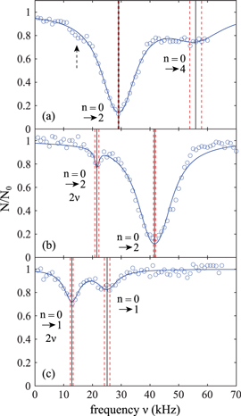
Figure 3. Amplitude ((a) and (b)) and phase (c) modulation spectra of weakly bound Feshbach molecules (a) and molecules in the rovibrational ground state of the  potential ((b) and (c)). We measure the fraction of remaining molecules
  as a function of the modulation frequency ν. The statistical error of each data point is in the range of
  . Here, the numbers N0 are given by the asymptotic limits of Lorentzian fits (solid blue lines). The resulting center frequencies of the resonances are illustrated as black vertical lines, while the red dashed lines indicate the corresponding uncertainties. We note, that the mean intensity of the lattice beam used for modulation in (b) is 30% less than in (a) and (c).
Download figure:
Standard image High-resolution imageNow, we turn to figure 3(c), which shows an excitation spectrum after phase modulation for va = 0 molecules. We observe two resonances of similar strength, both of which we assign to the transition from n = 0 to n = 1. The dip at lower frequency is again a subharmonic resonance. Surprisingly, it is stronger than the harmonic one at about 25 kHz. We attribute this to a purely technical issue, as the strength of the phase modulation varied with the frequency in our setup. However, we have verified the assignment of the resonances by comparison to the corresponding amplitude modulation spectra.
We calculate the Bloch bands by diagonalizing the Hamilton operator for the lattice in 1D (neglecting gravitation),

which is particularly simple in momentum space (see, e.g., [41]). Here, m is the mass of a molecule, i.e., twice the mass of a  atom. Figure 4 shows the calculated energy eigenvalues as a function of the lattice depth. The energies are given in terms of the recoil energy
  , with h being Planck's constant. As we do not specify the quasimomentum, the energy eigenvalues form bands which are broad for low lattice depths. However, the bands n = 0 to n = 2 are quite narrow for lattice depths above
  . This is the regime where we take most of our measurements. Having measured the resonant excitation frequencies after modulation we could in principle use figure 4 to read off the corresponding lattice depth
  . We refine this method and at the same time check for consistency as follows.

Figure 4. Energy band-structure with zero energy corresponding to the center of the lowest Bloch band. Solid lines are calculations for a single lattice direction, where the numbers 1–8 give the band index n. The data points are obtained excitation energies for  , stemming from amplitude (circles) or phase (squares) modulation spectroscopy. Red (blue) plot symbols indicate measurements for triplet rovibrational ground state (Feshbach) molecules. Here, the experimental results are shown after independently fitting the data for each molecular species to the band-structure calculation. By doing so, we determine the individual calibration factors and therefore the lattice depths
  (see also text). The horizontal error bars represent the resulting uncertainties of
  , whereas the vertical error bars are given by the uncertainties of the Lorentzian fits in the modulation spectra.
Download figure:
Standard image High-resolution imageIn the experiment we control the lattice depth  via the laser beam power P that can be measured using photodiodes. The square to the electrical field
  is proportional to P. Consequently
  , i.e., the precise value of
  is known up to a calibration factor (which depends linearly on the dynamical polarizability). Thus, given a molecular state, we should be able to adjust the calibration factor such that all data obtained for various powers P match the band-structure calculation. The measured data points in figure 4 clearly show that this works quite well, both for deeply bound molecules (red) and Feshbach molecules (blue). In this procedure we do not account for the transitions from n = 0 to n = 4 owing to the large uncertainties of the corresponding resonances in the excitation spectra. Nevertheless, these data points are shown in the plot for comparison.
In addition to  , the electrical field amplitude E0 of the optical lattice has to be determined in order to infer the dynamical polarizability
  (see equation (1)). We can circumvent this by referencing the measurements on the lattice depth
  for the molecules in the rovibrational ground state of the
  potential to similar measurements with Feshbach molecules, of which the polarizability
  is known to be twice the one of a Rb atom
  in the electronic ground state [18]. According to equation (1) the lattice depths
  and
and  for the va = 0 and Feshbach molecules are related by

for a given lattice beam intensity, i.e., a given E0.
From our experiments at  nm we obtain
  , whereas
  was found at
  [13]. Using our calculated atomic values of 685.8 (1064.5 nm) and 2995.9 a.u. (830.4 nm) yields molecular polarizabilities
  of 3430 ± 140 (1064.5 nm) and 600 ± 120 a.u. (830.4 nm), respectively.
5. Comparison of results
Table 1 shows our measured and calculated polarizabilities along with results of other references. First, it should be noted that our theoretical atomic polarizabilities (including only the 5s–5p and 5s–6p transition frequencies from the NIST database [42]) at 828.4 and at 1060.1 nm are in good agreement with the ones of [43, 44] which consider the 5s–5p transition frequency from the NIST database, and ab initio values for the frequencies up to the 5s–8p transitions.
Table 1. Measured and calculated polarizabilities  in a.u. for
  atoms and
  molecules in the rovibrational ground state of
  . Here, the abbreviations 'tw exp (theo)' mean 'this work, experimental (theoretical)'.
| Species |
 (nm) (nm) | Re  (a.u.) (a.u.) | Ref. |
|---|---|---|---|

| 828.4 |

| [43] |

| 828.4 | 3131.4 |
 theo theo |

| 830.4 | 2995.9 |
 theo theo |

| 830.4 | 875.8 |
 theo theo |

| 830.4 |
 
| [13], using a.u. a.u. |

| 1060.1 | 692.7 |
 theo theo |

| 1060.1 |

| [44] |

| 1064.5 | 685.8 |
 theo theo |

| 1064.5 | 3147 |
 theo theo |

| 1064.5 |

|
 exp, using exp, using a.u. a.u. |

| 1064.5 |

| [46] |

|

|

| [48] |

|

| 317.9 |
 theo theo |

|

| 698.5 |
 theo theo |

|

| 677.5 | [49] |
We find good agreement between our theoretical (3147 a.u.) and experimental (3430 ± 140 a.u.) results for the molecular polarizability  at 1064.5 nm (see table 1). In contrast, the agreement for the polarizability at 830.4 nm of our former measurements [13] (600 ± 120 a.u.) with the present calculations (
 ) is somewhat poor. In view of this discrepancy we want to estimate the influence of slight shifts of the PECs on the calculations. The potential well depths of the
  and the
  states used in the computation are smaller by 72 and
  with respect to the experimental determinations of [29] and [30], respectively. Such shifts would lead to a change in the calculated polarizability of about 10% for the particular wavelengths of 830.4 and 1064.5 nm. This sets a range for the uncertainty of the calculated polarizability that arises from the uncertainty of the PECs. Furthermore, in terms of the experiments, we note that in [13] a different method to determine the dynamical polarizability was used. The polarizability was inferred from the oscillating dynamics of molecular wave packets that occurred when v = 0 molecules were suddenly loaded into several Bloch bands of the optical lattice. This leaves potentially room for a systematic discrepancy between the two measurements. With respect to the static polarizability, i.e.,
  , the calculations presented in this work give 698.5 a.u. (cf table 1) for the va = 0 molecules. This value actually agrees well with the one previously reported in [49], 677.5 a.u., as it was not including the contribution of
  a.u. [45].
Figure 5 is a zoom into figure 1(b) showing the calculated real part of the dynamical polarizability of a  molecule (solid black lines). In addition,
  for a Feshbach molecule is plotted (dashed red lines), which is given by twice the atomic polarizability. The two wavelengths used in our experiments (830.4 and 1064.5 nm) are indicated as vertical green dashed lines. Outside the resonant and therefore lossy regions in figure 5 (vertical black bands) the two polarizability curves never cross. Thus, there is no so-called 'magic' wavelength, where the ac Stark shift of the two molecular states caused by the trapping light is equal. Such state-insensitive trapping conditions can be beneficial, e.g., when converting Feshbach molecules to deeply bound states. Specifically, in [13], owing to the large difference of the dynamical polarizabilities at
  nm, the STIRAP transfer of
  from the Feshbach level to
  populated several lattice bands.
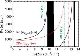
Figure 5. Real parts of the dynamical polarizabilities of triplet rovibrational ground state molecules (solid black lines) and Feshbach molecules (dashed red lines). The circles represent the experimental results given in table 1 with the corresponding wavelengths indicated by green dashed vertical lines.
Download figure:
Standard image High-resolution imageWe have again studied this issue in this work and find that population of higher lattice bands can be suppressed even in the absence of a magic wavelength when working with deep lattices. At  nm there is still a factor of 2.5 difference in polarizability between Feshbach and
  = 0 molecules. For an initial (final) lattice depth of
  ) at 1064.5 nm a calculation of the wave function overlap for the Bloch states shows that still
  of the population stays in the lowest Bloch band after the STIRAP. In addition, we are able to energetically resolve the lattice bands during STIRAP as n = 0 and n = 2 are separated by about 40 kHz at
  (cf figure 4). This strongly increases the selectivity of the transition (see, e.g., [50]). Indeed, in our experiments we do not observe any significant population of higher bands.
As can be seen in figure 5, the absolute dynamical polarizability of the triplet rovibrational ground state molecules at  is about four times larger than at
  . This is convenient since it results in a four times deeper interaction potential at the same laser intensity. For longer wavelengths than
  , figure 5 reveals, that the dynamical polarizabilities of va = 0 molecules and Feshbach molecules approach each other. Hence working at even longer wavelengths than 1064.5 nm might be advantageous for some applications.
6. Lifetime of the molecules
According to equation (2), the imaginary part of the dynamical polarizability, Im  , is linked to the light power absorbed by a molecule, Pabs, which in turn can be expressed in terms of the photon scattering rate
  [21]. Using this and equation (1),
  can be written as

For a 3D optical lattice with equal lattice depths  in each direction the scattering rate is given by
  . As an example, we consider the case of
  at
at  . Then, the corresponding values for the polarizability obtained in the present work,
  and
and  , yield
  . Note, this calculation only accounts for an ideal optical lattice. As there is always background light that does not contribute to the lattice, the estimated value for the scattering rate represents just a lower bound. Once a photon is absorbed, the molecule is excited and typically decays to a nonobservable state. Assuming excitation to be the only loss-mechanism a lifetime
  of the va = 0 molecules is expected in a
  deep 3D optical lattice at
  .
.
We experimentally investigate the lifetimes of the molecules in the rovibrational ground state of  by varying the holding time th in the lattice. Figure 6 shows lifetime measurements of va = 0 molecules for various potential depths
  , which are adjusted to be equal in each direction. Applying an exponential fit, we obtain a
  decay time τ of more than
  for both our measurements at
  and
and  .
.
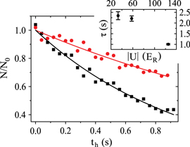
Figure 6. Decay of triplet rovibrational ground state molecules trapped in a 3D optical lattice at  with equal potential depths
  in each direction. Shown is the fraction of remaining molecules
  as a function of the holding time th in the lattice. Square plot symbols (red circles) correspond to a lattice depth of
  (
( ). Each data set typically consists of 10–15 repetitions of the experiment, where the statistical error of a data point is on the order of ±0.1. Solid lines are exponential fits to the data. Here, N0 is given by the values of these fits at
  . In general, the absolute molecule numbers N0 are about
  . The inset depicts the resulting
  decay times for various lattice depths.
Download figure:
Standard image High-resolution imageIn order to estimate possible loss induced by inelastic molecular collisions, we calculate the tunneling rates  between adjacent lattice sites within the lowest Bloch band (n = 0). When considering a lattice depth of
  (
( ) one obtains
  (
( ). In our setup at most 20% of the lattice sites are occupied in the region of highest molecule density. Thus, for
  decay due to collisions cannot be neglected, whereas for
  and beyond the only relevant loss mechanism is photon scattering. For such deep lattices, the lifetime τ scales directly inversely with the lattice depth
  . We confirm this for the measurements at
  and
and  , since the ratio of the lifetimes
  is close to
  .
.
7. Polarizability of molecules

As the agreement between calculations and measurements for the triplet molecules is in general good, we also provide calculations for the singlet ground state of  . Using the same approach as above (see also [18]), we compute the dynamical polarizability
  , i.e., with respect to the vX=0,
  level. The
  PEC has been derived from spectroscopic data of [51]. The
  and the
  PECs and the related spin–orbit coupling between those two states are taken from [52]. The PECs for all the other states and for the TEDMs are taken from the computations reported in [23, 24]. Again, the sum in equation (3) has been truncated to include only the levels of the four lowest
  states and the three lowest
  states. The natural lifetime of the excited levels has been fixed at 10 ns. Results are presented in figure 7, showing that two magic wavelengths can be identified at 990.1 and 1047.2 nm. The latter is located close to the region of strong absorption resonances and consequently, from the imaginary part (cf figure 7(b)), the photon scattering rate at 1047.2 nm is expected to be about four times larger than at 990.1 nm.

Figure 7. Real part (a) and imaginary part (b) of the dynamical polarizability of 
 molecules in their vX = 0, N = 0 level. In (a), for comparison, also the numerical results corresponding to
  are shown (red dashed line), representing the real part of the dynamical polarizability of Feshbach molecules. Two magic wavelengths, where both polarizabilities are equal, are obtained and indicated by vertical dashed lines.
Download figure:
Standard image High-resolution image8. Parametrization of the polarizability
8.1. Rovibrational ground state of

In general, using figures (e.g., figures 1 and 7) to read off the dynamical polarizabilities at specific wavelengths is cumbersome. Therefore, we provide here a simple analytical fitfunction and parameters that allow for reproducing the numerical results with respect to nonresonant wavelength regimes. In the infrared and optical domain we are studying, the main contributions to the polarizability of the X (a) state outside of resonances come from the transitions toward the first excited  state and the first
  state. Thus we attempt to model the polarizability by reducing those transitions to a single effective transition toward each of the two different symmetries. The approximate real part of the polarizability is expressed as

with  (resp.
  ) the effective transition frequencies and
  (resp.
  ) the corresponding effective dipole moments. We have isolated in this expression the core polarizability
  as its frequency dependence is much weaker than the one of the terms coming from valence electron excitation (see appendix
We extract the effective parameters from a fit to the full numerical results using equation (8). The results with respect to the  and
and  rovibrational ground state are shown in figure 8. For the triplet case, data points with frequencies close to resonances, i.e., from
  to
to  and above
  , are excluded from the fit. We obtain
  ,
,  ,
,  and
and  Note, in terms of dipole moments, a.u. can be converted into SI units according to
  . Using these parameters, the effective polarizability reproduces the numerical results in the fitted region to within a relative root mean square value (rRMS) of around 1% (see figure 8(a)). The rRMS value is defined by

with  being the numerical values, and
  the fitted ones. Here, M is the number of considered values
  , which depends on the vibrational level as the resonant frequency regions excluded from the fit vary. We point out that if we take the transition dipole moment dZ (resp. dX = dY) at the equilibrium distance of the
  state and multiply it by the appropriate Hönl–London factor (
 for
for  transition and
  for
for  transition), we get the value
  (resp. 3.142 a.u.), very close to the effective dipole moment found above. Moreover, the effective transition frequencies correspond roughly to the average frequencies of transitions with favorable Franck–Condon factor.

Figure 8. Analytical fits of the dynamical polarizabilities of the  molecule in va = 0, N = 0 (a), and of the
  molecule in vX = 0, N = 0 (b). Frequency ranges excluded from the fits are indicated as shaded areas. At the scale of the figure, the original curves and the fitted curves are indistinguishable.
Download figure:
Standard image High-resolution image8.2. Rovibrational ground state of

A similar fit can be performed for the dynamical polarizability of  molecules in the (vX = 0, N = 0) level (figure 8(b)). Frequency domains from
  to
to  , from
  to
to  and above
  , corresponding to resonances toward the
  ,
,  and
and  excited states, respectively, were excluded from the fit. We omitted to account for levels of the
  state as they have a very small singlet character. Then, the fit to the numerically calculated dynamical polarizability yields
  ,
,  ,
,  and
and  Again, we point out that the effective transition dipole moments obtained are very close to the electronic transition dipole moments taken at equilibrium distance multiplied by the Hönl–London factors, i.e., 2.613 and
  , respectively. Here, the rRMS of the fit is 0.5%.
8.3. Excited vibrational states
Both, the frequency domains with good Franck–Condon factors and transition dipole moments depend significantly on the initial vibrational level. This is reflected in the variation of the effective parameters when we perform an individual fit for each vibrational level (with N = 0) of the  (va = 0–40) and
  (vX = 0–124) states. The corresponding parameters, which can be used to reproduce the dynamical polarizabilities in the nonresonant frequency domains, are reported in the supplemental material (see footnote 3). Figure 9 shows the resulting rRMS values as a function of the vibrational level with respect to the lowest triplet and singlet state.

Figure 9. Relative root mean square (rRMS) values of the analytical fits to the numerically calculated dynamical polarizabilities. Blue closed (red open) circles correspond to fit results obtained with the 'two-effective-transitions' ansatz for the vibrational levels va of  (vX of
  ), whereas the black closed squares stem from fits including a third effective transition to represent the dynamical polarizabilities with respect to va, which significantly increases the accuracy (see text). The rRMS values for
  do not exceed 0.1% (not shown here).
Download figure:
Standard image High-resolution image
Figure A1. Computed transition electric dipole moments (TEDMs) for the main transitions from the  and the
  states to the states correlated to the 5s + 5p dissociation limit (a), the 5s + 4d dissociation limit (b), the 5s + 6s dissociation limit (c), and the 5s + 6p dissociation limit (d). The individual curves can be assigned to the corresponding transitions as indicated on top of the graph using the numbers i and j. At large distances the TEDMs converge toward
  which is equal to the atomic TEDMs multiplied by
  (see text).
Download figure:
Standard image High-resolution imageUsing the ansatz of equation (8) gives a poor result for most excited vibrational levels of the  potential with an rRMS exceeding 4% in the range of va = 2–27. This behavior is related to the fact that Franck–Condon factors mainly depend on the amplitude of the excited wave function around both the inner and the outer classical turning points of the initial vibrational level studied. The shape of the
  potential is quite different compared to the relevant excited states. Consequently, the inner turning point region of a given vibrational level va will induce couplings to levels of excited molecular states with energies strongly different from those related to couplings induced by the outer turning point region. This effect mainly occurs for the excited
  potential wells as they are deep. Instead, the depth of the
  potential is not sufficient to create such a variation.
Thus we added one more transition term to the ansatz of equation (8) in order to account for both the inner and outer part of the  –
– transitions in the model. This reduced significantly the rRMS of the effective polarizabilities of the va levels (see figure 9). We want to emphasize that such an interpretation gives a reasonable physical picture for most levels. However, for some levels like the deeply bound ones or those close to the dissociation limits, the three-effective-transition model is somewhat artificial and the effective parameters should be taken only as numerical parameters needed to easily obtain the corresponding polarizability.
9. Conclusion
We have studied the dynamical polarizability of the 87Rb2 molecule in the rovibrational ground state of the  potential. Calculations of both, the real and imaginary part are provided and we measured
  at
at  . Our experimental and theoretical findings show good agreement. From our computed value of
  at this wavelength, we expect trapping times of the molecules on the order of seconds for lattice depths around
  , which was confirmed by our observations. We also have investigated theoretically the dynamical polarizability of the singlet ground state
  . These results are interesting for future STIRAP transfer of Rb2 to the corresponding rovibronic ground state. Furthermore, we have introduced a simple analytical expression to parametrize the dynamical polarizabilities for all levels of both,
  and
and  states. By fitting this expression to the numerical results, we have extracted effective parameters, which can be used to reproduce
  of a given vibrational state with high fidelity. The precise knowledge of the dynamical polarizability enables accurate control of optical dipole potentials and therefore is of importance for future experiments with deeply bound Rb2 molecules.
Acknowledgments
This work was funded by the German Research Foundation (DFG). RV acknowledges partial support from Agence Nationale de la Recherche (ANR), under the project COPOMOL (contract ANR-13-IS04-0004-01).
Appendix
A.1. Polarizability of the core

As the two ionic  cores are only weakly perturbing each other, we consider the molecular core polarizability as twice the atomic
  polarizability. First, we calculate the atomic polarizabilities at imaginary frequencies
  [53], which includes only the contribution of the valence electron. We subtract them from the values of [21], where the resulting differences represent the contribution of the core electrons, and thus the
  polarizability. Following [21] this estimate assumes that the influence of the valence electrons on the core polarizability is negligible.
We use an ansatz similar to the one of equation (8) to model the core polarizability with two effective transitions. This yields the effective frequencies  and
and  , and the effective dipole moments 2.72799 and 1.40119 a.u. We note that these two transition frequencies are on the order of magnitude of the main transition in
  and
and  , respectively. The core polarizability is a small contribution slowly varying from
  at vanishing frequency up to
  in the optical domain relevant here. For the static case, we can compare the result of our calculations to the value of
  reported in [45] and find good agreement.
A.2. TEDMs
For the sake of completeness we show in figure A1 the TEDMs included in the calculations of the dynamical polarizabilities as functions of the internuclear distances. The corresponding numerical values are given in the supplemental material (see footnote 3). Some of the data with respect to the lowest transitions have already been reported in [23, 24]. The largest TEDMs in the range of the PECs concern the first excited  and Π potentials (see figure A1(a)). At large distances the molecular excited electronic wave functions become close to the form
 ![$[{\phi }_{5{\rm{s}}}(1){\phi }_{{nl}}(2)\pm {\phi }_{5{\rm{s}}}(2){\phi }_{{nl}}(1)]/\sqrt{2}$](https://content.cld.iop.org/journals/1367-2630/17/6/065019/revision4/njp515397ieqn383.gif) and therefore the TEDMs converge toward
and therefore the TEDMs converge toward  , which is equal to the atomic TEDMs multiplied by
  . We find
  a.u. and
  a.u., in excellent agreement with the values extracted from the NIST database [42] (4.226 and 0.3531 a.u.), obtained by averaging the TEDMs corresponding to
  and
and  for n = 5 and 6, respectively. This confirms the good quality of the present representations of the atomic electronic wave functions.
Footnotes
- 3
See supplemental material available at stacks.iop.org/njp/17/065019/mmedia for the results of the analytical fits to the calculated polarizabilities corresponding to different vibrational levels va (vX) of
() using two or three effective transitions and for the numerical values of the transition electric dipole moments starting from either the lowest triplet state () or singlet state () toward the most relevant excited potentials.


