


Abstract
The thermodynamic entropy production for the scattering processes of noninteracting bosons and fermions in mesoscopic systems is shown to be related to the difference between the Connes–Narnhofer–Thirring entropy per unit time, characterizing temporal disorder in the motion of quantum particles, and the associated time-reversed coentropy per unit time. Under nonequilibrium conditions, the positivity of thermodynamic entropy production can thus be interpreted as a time-reversal symmetry breaking in the temporal disorder of the quantum transport process. Moreover, the full counting statistics of both fermionic and bosonic quantum transport is formulated in relation with the energy and particle currents producing thermodynamic entropy in nonequilibrium steady states.
Export citation and abstract BibTeX RIS

Content from this work may be used under the terms of the Creative Commons Attribution 3.0 licence. Any further distribution of this work must maintain attribution to the author(s) and the title of the work, journal citation and DOI.
1. Introduction
At positive temperature, atoms and molecules undergo ceaseless collisions and their motion is highly irregular, manifesting fluctuations on micrometric and nanometric spatial scales, as illustrated with Brownian motion. The characterization of this dynamical randomness or temporal disorder is a major preoccupation in this context. Already the fluctuation-dissipation theorem [1] holding in regimes close to thermodynamic equilibrium shows that energy dissipation is related to the stochasticity of motion at equilibrium. In the eighties, work on dynamical chaos has developed new concepts such as the Kolmogorov–Sinai (KS) entropy per unit time, which characterizes temporal disorder in deterministic dynamical systems [2–6]. This quantity represents the rate of information production by a measurement device recording bits of information on the system history. The KS entropy per unit time is related to the Lyapunov exponents characterizing the sensibility to initial conditions and to the escape rate of trajectories from open systems [5, 6]. This latter quantity is proportional to transport properties such as diffusion, viscosity, or heat conductivity, which establishes fundamental relationships between irreversibility and the characteristic quantities of microscopic chaos [7–10]. Since then, similar dynamical large-deviation relationships have been found for different types of systems. For stochastic systems such as Brownian motion or Markovian jump processes, the KS entropy per unit time is infinite because randomness is supposed to manifest itself on arbitrarily small space or time scales in such processes. Therefore, it is required to introduce the spatial ( ) or temporal (τ) resolution, at which the process is observed, and to characterize its dynamical randomness with an (
 )-entropy per unit time [10, 11]. This quantity reduces to the KS entropy per unit time in chaotic deterministic systems. For stochastic processes such as Brownian motion or Markovian jump processes, the (
 )-entropy per unit time increases with the resolution as
  or
or  and it can be experimentally measured from time series [11, 12]. Such dynamical large-deviation quantities allow us to characterize the chaotic properties of temporal disorder in different types of stochastic systems [13–15].
A time-reversed coentropy per unit time can also be introduced to characterize temporal disorder in the time reversals of the typical histories followed by the system [16–19]. This quantity is called a coentropy because it forms a nonnegative Kullback–Leibler divergence if combined with the corresponding entropy [20, 21]. Remarkably, the difference between the time-reversed coentropy and the entropy per unit time is related to the thermodynamic entropy production, showing that the time-reversal symmetry is broken for the temporal disorder of nonequilibrium processes [16–19]. This relationship has been used in an experimental study of driven Brownian motion and electric noise, which revealed the time asymmetry of nonequilibrium temporal disorder on scales as small as a few nanometers for the position of the Brownian particle, or a few thousands of electron charges transferred in the electric circuit [22, 23]. In regard of the fundamental and practical importance of understanding the origins of irreversibility, we may wonder if such results could be extended to other nonequilibrium systems as well.
The purpose of the present paper is to demonstrate that the relationship between the time asymmetry of temporal disorder and the thermodynamic entropy production can also be established for many-body quantum systems of noninteracting bosons or fermions. In the eighties, Connes, Narnhofer, and Thirring (CNT) have introduced a quantum generalization of the classical KS entropy per unit time to characterize temporal disorder in quantum systems [24]. The CNT entropy per unit time is positive only for many-body quantum systems and their analytical expression has been deduced for many-body systems of noninteracting bosons or fermions [25–29]. In this context, the entropy production is also expected to result from the comparison between the probabilities of the system histories and their corresponding time reversals [30]. It is therefore natural to associate a time-reversed coentropy to the CNT entropy per unit time, as recently proposed for the one-dimensional scattering of fermions [19].
Here, our aim is to extend these considerations to general scattering processes of fermions and bosons in multiterminal mesoscopic circuits. This concerns not only quantum electronic transport in mesoscopic semiconductor devices [31, 32], but also the quantum transport of neutral matter since the quantization of conductance has been recently observed for ultracold atomic fermions flowing through a tiny constriction in an optical trap [33]. This constriction is a scatterer in the quantum wire connecting two reservoirs. If the two reservoirs have different chemical potentials or temperatures [33, 34], the ultracold atoms are out of equilibrium and irreversibility manifests itself, as previously shown for single-electron transport [35]. This irreversibility is characterized by entropy production. Here, it is shown that entropy production in the flow of noninteracting fermions or bosons can be expressed in terms of the time asymmetry in the nonequilibrium temporal disorder characterized by the CNT entropy per unit time and its associated coentropy.
Furthermore, the full counting statistics is established for both fermionic and bosonic neutral atoms, which allows us to confirm the expression of entropy production in terms of the mean energy and particle currents between the reservoirs.
The paper is organized as follows. In section 2, the scattering approach to quantum transport is briefly presented. The CNT entropy per unit time and its associated time-reversed coentropy are introduced, as well as the thermodynamic entropy production and the full counting statistics. The announced relationships are established for fermions in section 3 and for bosons in section 4. Conclusions are drawn in section 5.
2. Temporal disorder, time reversal, and entropy production
2.1. Scattering in a mesoscopic circuit
We consider the ballistic motion of noninteracting particles in a multiterminal mesoscopic circuit connecting several particle reservoirs. The particles carry energy so that the transport of particles induces the transport of energy between the reservoirs  (where r is the number of terminals and reservoirs). The circuit is described by the energy potential
  that is common to every particle, where
  is the position of the particle in a d-dimensional space. The particles have the mass m and the spin s. The Hamiltonian operator describing the many-body quantum dynamics is given by

in terms of the creation-annihilation field operators,  and
and  , obeying the canonical commutation or anticommutation relations

whether the particles are respectively bosons if their spin is integral, or fermions if their spin is half-integral. The spin multiplicity is  . We suppose that there is no external magnetic field so that the Hamiltonian operator is symmetric under time reversal
  :
:

For spinless particles, the time-reversal operator  takes the complex conjugate of the wavefunction.
As depicted in figure 1, the mesoscopic circuit has several terminals of infinite spatial extension. In every terminal  , there exist spatial coordinates
  where
where  is the coordinate parallel to the axis of the terminal and
  are the perpendicular coordinates. The energy potential is asymptotically independent of the spatial coordinate
  in the direction of the terminal

where  is the profile of the potential transverse to the terminal l, which constitutes a waveguide. Asymptotically in this waveguide, the stationary states of the one-body Hamiltonian operator

can be written as

where p is the momentum in the direction of the waveguide l,  are
are  quantum numbers labeling the modes transverse to the waveguide, and
  a spinorial amplitude with
  . The different transverse modes are so many possible channels for transport. The corresponding energy eigenvalues are given by

where  is the energy threshold for the opening of the channel
  .
.
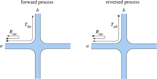
Figure 1. Schematic representation of a four-terminal circuit comparing the forward scattering process from channel  to channel
  (left-hand side) with the corresponding reversed process (right-hand side). Tba is the transmission probability from a to b and Raa is the reflection probability from a back to a.
Download figure:
Standard image High-resolution imageThe terminals join together in a cavity, which forms the scatterer. In every terminal, the parallel coordinate  increases towards the scatterer so that the incoming waves have a positive momentum
  and the outgoing waves a negative one
  (if the energy is large enough
  ). As shown in scattering theory [31, 32, 36, 37], the probability amplitude of the incoming wave
  is linearly transformed into the amplitude of the outgoing wave
  by the scattering matrix
  , which is unitary. If we define the probabilities of reflection in the channel a and of transmission from the channel a to the channel b by


the unitarity of the scattering matrix implies that

For spinless particles or for a process without spin flip, the matrix elements of the scattering matrix do not depend on the spin and the time-reversal symmetry implies that the scattering matrix is equal to its transpose [31]. As a consequence, the transmission probabilities satisfy

Now, the energy of the particles incoming in the channel  has the equilibrium statistical distribution of the
  reservoir at the inverse temperature
  and the chemical potential
  (where
  denotes Boltzmann's constant). For bosons or fermions, the mean occupation numbers of the incoming states are respectively given by the Bose–Einstein or Fermi–Dirac distribution,
  [38, 39]. We notice that the chemical potentials of the reservoirs depend on their internal mean particle density
  and temperature Tl according to equilibrium relations that are specific to the reservoirs:
  .
.
Under nonequilibrium conditions, the reservoirs have different inverse temperatures or chemical potentials. Consequently, the forward path from the channel  to the channel
  does not have the same probability as the reversed path from the channel
  to the channel
  . Indeed, the forward path is weighted by the mean occupation number of the incoming reservoir l, which concerns the reflected path
  and the transmitted path
  . The reflected path is mapped onto itself by time reversal and, thus, it does not change its probability weight. In contrast, the transmitted path is mapped onto
  , which is now incoming from the reservoir k that has a weight determined by its own mean occupation number fk, as schematically depicted in figure 1. The key point is that the mean occupation numbers differ
  away from equilibrium because the reservoirs have different temperatures or chemical potentials. This important observation shows that the time-reversal symmetry is broken at the level of the statistical description, although the time-reversal symmetry (3) always holds for the microscopic dynamics. Such symmetry-breaking phenomena are well known in condensed-matter theory for spin-reversal or rotational symmetries [40]. For nonequilibrium steady states, it is the time-reversal symmetry that is broken.
2.2. Temporal disorder in the forward and reversed processes
Here, our aim is to characterize the temporal disorder of the transport process of particles between the reservoirs. The forward process is observed during a time interval ![$[0,t]$](https://content.cld.iop.org/journals/1367-2630/17/4/045001/revision1/njp510954ieqn50.gif) with
with  . Particles are incoming from the channel a with their momentum between
  and
and  and they are scattered to the channel b with probability
  at the energy (7). In the incoming channel a, their velocity is given by
  so that they travel a distance
  . In this incoming channel, the number of possible one-body states
  that can be occupied by a particle of momentum in the interval
 ![$[p,p+\Delta p]$](https://content.cld.iop.org/journals/1367-2630/17/4/045001/revision1/njp510954ieqn58.gif) is given by
is given by

among which a fraction  is scattered into the channel b. Therefore, the number of possible states coming from the channel a and going to the channel b at the energy is evaluated as

The occupation of these states is fixed by the mean occupation number  of the incoming reservoir l for the channel
  , whereupon the average number of particles transported on the
  one-body states is given by

The number n of particles occupying a given state j is a random variable with a probability distribution Pj(n), which is known for bosons and fermions (see below). For fermions, the only possible values of this number are n = 0, 1 because of Pauli's exclusion principle. For bosons, this number can take any integer value,  The mean occupation number is related to the probability distribution Pj(n) according to
  .
.
Let us denote by α the one-body paths from the channel a to the channel b with a momentum in the interval ![$[p,p+\Delta p]$](https://content.cld.iop.org/journals/1367-2630/17/4/045001/revision1/njp510954ieqn65.gif) ,
,  the number of possible one-body states with the corresponding energy (7) following the path α, and
  the number of particles occupying all these states. This latter is the sum of the random occupation numbers of every state in the set
  of the
  possible states:
  . A history
  followed by the many-body system during the time interval
 ![$[0,t]$](https://content.cld.iop.org/journals/1367-2630/17/4/045001/revision1/njp510954ieqn72.gif) is specified by the set of random numbers
is specified by the set of random numbers  of the particles occupying all the possible states. Since the different states are occupied independently of each other, the probability of the history
  factorizes as

For such a process, the temporal disorder is characterized by the entropy per unit time

This quantity is the mean exponential decay rate of the history probability:  . Inserting the factorization (15), we find that

Separating the states  into the aforementioned classes
  , we get

Since all the states in the class  have approximately the same energy and thus the same probability distribution
  for all
  , the entropy per unit time has the following expression

because  for
for  given by equation (13). This entropy per unit time is always nonnegative
  and it can be interpreted as the rate of information production in the recording of typical histories.
A time-reversed coentropy per unit time can be defined by considering the probability of the reversed history  . For the reversed process, the probability weight of a path is determined by the mean occupation number of the reservoir, from which the reversed path is issued. For the path α from channel a to b, the reversed path is coming from the reservoir b and its mean occupation number is fb. If the probability distribution
  of the forward path corresponds to the mean occupation number fa, the probability distribution
  of the reversed path corresponds to the mean occupation number fb. The probability of the reversed history is thus given by

For a typical history  of the forward process, the probability (20) is also exponentially decaying, but at a rate
  different from the one (19) of the probability
  . Averaging with respect to the forward process, we define the time-reversed coentropy per unit time

By the same reasoning as above, the coentropy is thus given by

2.3. Thermodynamic entropy production
In analogy with other processes [16–19, 22, 23], the thermodynamic entropy production can be defined as the difference between the time-reversed coentropy and entropy per unit time as

This difference forms a Kullback–Leibler divergence, which is known to be always nonnegative [20, 21], as it should for the entropy production obeying the second law of thermodynamics. We notice that  . The equality
  holds if the system is at equilibrium and the principle of detailed balance is satisfied, in which case the entropy production is vanishing.
In the following sections, we shall show that the definition (23) leads to the standard expression of the thermodynamic entropy production:

in terms of the average values of the energy and particle currents,  and
and  , from the reservoir l to the reference reservoir r, and the affinities or thermodynamic forces:


2.4. Full counting statistics and entropy production
In the following, we shall also obtain the cumulant generating function of the currents characterizing the full counting statistics for the transport of noninteracting bosons and fermions. The first cumulant should give the average values of the currents and, thus, the thermodynamic entropy production (24), which is a further check of the results.
As previously shown [46–48], the cumulant generating function can be obtained in the two-measurement scheme. The energy and particle contents of the reservoirs can be measured before the initial time t = 0 when the reservoirs were decoupled. The interaction between the reservoirs is switched on during the time interval extending until  , after which the interaction is switched off and the energy and particle numbers can again be measured in the decoupled reservoirs. During the interaction period, the Hamiltonian operator is given by
  . In this scheme, the energy and particle numbers transferred between the reservoirs can be measured and their probability can be calculated. The generating function of the statistical moments is given by

in terms of the counting parameters  , and the time-evolved Hamiltonian and particle-number operators of the reservoirs:


where  is the unitary evolution operator induced by the total Hamiltonian
  . The averaging is carried out over the initial density operator of the total system

where  is the grand-canonical partition function of the
  reservoir,
  its inverse temperature, and
  its chemical potential.
The cumulant generating function is thus defined as

In particular, the average values of the currents flowing from the reservoir l to the sink taken as the reference reservoir r are given by


for  . We notice that the time-reversal symmetry (3) has for consequence the symmetry relation

as proved elsewhere [46–48]. Equation (34) is the expression of the multivariate exchange fluctuation theorem [49–56].
For independent particles, every many-body operator can be expressed in terms of the corresponding one-body operator, as in equation (1). A formula obtained by Klich [57] allows us to reduce the calculation of the cumulant generating function from the many-body to the one-body problem. For fermions, this calculation leads to the Levitov–Lesovik formula [58], the analogue of which is obtained here below for bosons. Consequently, the average values of the currents can be found and the expression (24) of the entropy production can be deduced equivalently from the definition (23) and the cumulant generating function, for bosons as well as fermions. These are the purposes of the following sections.
3. Transport of fermions
3.1. Temporal disorder in the forward and reversed processes
For fermions, the mean occupation number is given by the Fermi–Dirac distribution

in each reservoir  at the inverse temperature
  and chemical potential
  . According to Pauli's exclusion principle, a given one-body state
  is either occupied or not, so that its occupation number takes the values n = 0,1. In the equilibrium grand-canonical ensemble, the probability distribution of the occupation number is defined by

implying  .
.
Consequently, the entropy per unit time (19) is given by

where the sum extends over the paths  at the energy . The same result can be obtained by supposing that
  fermions occupy the
  possible states. According to the fermionic statistics [38, 39], the number of possible histories is evaluated as

which is growing exponentially in time at the rate (37).
For the forward process, the Fermi–Dirac distribution is the one of the reservoir l, from which the particles are incoming in the channel  :
:  . The sum over the final reservoir b simplifies by the unitarity of the scattering matrix:
  . Finally, the sum over the momentum intervals
 ![$[p,p+\Delta p]$](https://content.cld.iop.org/journals/1367-2630/17/4/045001/revision1/njp510954ieqn116.gif) becomes the integral
becomes the integral

over the energy spectrum beginning at the threshold  of the channel
  . Therefore, the entropy per unit time characterizing the temporal disorder of the forward process is obtained as

where the sum extends over all the channels  of all the terminals
  . Equation (40) is the expression of the CNT entropy per unit time introduced in [24, 25]. An important property is that the CNT entropy of a quantum process does not depend on the resolution used to observe the temporal disorder, contrary to the situation for stochastic processes. The reason is that the quantum-mechanical states correspond to the limiting resolution
  , so that the temporal disorder is bounded to a maximum value. At low temperature or high chemical potential
  , the CNT entropy per unit time (40) vanishes as

if there is a single open channel in every terminal, which shows that the temporal disorder disappears as the temperatures of the reservoirs are vanishing. The CNT entropy per unit time (40) for r = 2 reservoirs is shown in figure 2 as a function of the common temperature  for different values of the chemical potentials at thermodynamic equilibrium
  . As expected, the temporal disorder of the fermionic gas is vanishing at zero temperature.
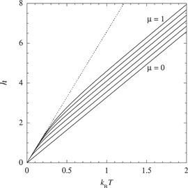
Figure 2. The temporal disorder of a fermionic gas in a single open channel of energy threshold  between r = 2 reservoirs characterized by the CNT entropy per unit time (40) in units of
  versus the thermal energy
  for the chemical potentials
  . The dashed line represents the limit (41). We notice that the CNT entropy takes half the value (41) if the chemical potentials are vanishing
  .
.
Download figure:
Standard image High-resolution imageNow, the time-reversed coentropy per unit time is calculated likewise from equation (22) as

where the Fermi–Dirac distribution to be considered for the reversal of the path  is
is  associated with the reservoir k of the channel
  . Here, the sum over the paths α remains a double sum over the incoming and outgoing channels a and b because there is no simplification of the sum over the outgoing channels b. We thus obtain
3.2. Thermodynamic entropy production
Now, the difference between the coentropy (43) and the entropy (40) per unit time can be evaluated by using the relation (10) due to the unitarity of the scattering matrix in order to decompose the entropy (40). The terms involving the reflection probabilities Raa are common to both quantities and are thus eliminated. We get

Since the Fermi–Dirac distribution has the property

the difference becomes

By using the sum rule  resulting from the unitarity of the scattering matrix, we can identify the average values of the energy and particle currents as


as it should according to the Landauer–Büttiker formulas [31, 32]. Therefore, the difference (46) can be written as

By the conservations of energy and particles


the currents of the reference reservoir r can be expressed in terms of the currents of the other reservoirs and we find

which is indeed the standard expression of the thermodynamic entropy production (24) in terms of the thermal and chemical affinities (25)–(26), as expected for quasi-free fermions [59–61]. This calculation demonstrates that the thermodynamic entropy production of quantum transport results from a time asymmetry in the temporal disorder characterized in terms of the CNT entropy and coentropy per unit time.
3.3. Full counting statistics and entropy production
For noninteracting fermions, Klich's formula

relates the many-body operators  and
and  to the corresponding one-body operators
  and
and  [57]. Accordingly, the moment generating function (27) can be expressed in terms of the one-body Hamiltonian and particle-number operators. In the limit
  defining the cumulant generating function (31), the one-body operators are decomposed onto the energy spectrum of the asymptotic noninteracting Hamiltonian and the scattering matrix
  is used to describe the effects of long-time evolution [48, 62]. Consequently, the cumulant generating function of all the fermionic currents is given by

in terms of the diagonal matrix  formed with the Fermi–Dirac distributions associated with every channel, and the diagonal matrices
  formed with the exponential functions of the counting parameters
  [58]. The time-reversal symmetry of the scattering matrix implies that the generating function (54) obeys the symmetry relation (34) so that the multivariate exchange fluctuation theorem holds [48].
The generating function (54) is depicted in figure 3 for the sole particle current between two terminals due to the scattering on a delta barrier. The system is isothermal and driven out of equilibrium by the difference of chemical potentials between both reservoirs connected to the terminals. The plot confirms the symmetry  of equation (34) with respect to the chemical affinity
  , which is the consequence of microreversibility (3).
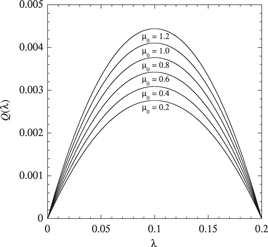
Figure 3. The cumulant generating function  versus the counting parameter
  for the fermionic current across the delta barrier
  between two reservoirs at the chemical potentials
  with
with  and varying
  . The other parameter values are
  ,
,  , and
, and  . The transmission probability of the delta barrier is given by
  . The chemical affinity takes the value
  .
.
Download figure:
Standard image High-resolution imageThe calculation of the first cumulants by taking the partial derivatives of the generating function (54) with respect to the counting parameters according to equations (32) and (33) gives the following expressions for the energy and particle currents


which are equivalent to equations (47) and (48) [32], confirming again the demonstration of the thermodynamic entropy production.
4. Transport of bosons
4.1. Temporal disorder in the forward and reversed processes
For bosons, the mean occupation number is given by the Bose–Einstein distribution

for  [38, 39]. The chemical potentials should be lower than or equal to the minimum energy of the spectrum:

Indeed, the Bose–Einstein distribution diverges at  due to the phenomenon of condensation, which happens at
  . Here, we only consider the transport of uncondensed particles so that we suppose that
  in every channel and leave open the issue of condensate transport.
In a bosonic system, the occupation number of any one-body state  is an arbitrarily large integer:
  . In the equilibrium grand-canonical ensemble, the probability distribution of the occupation number is given by

so that  [39].
[39].
Accordingly, the CNT entropy per unit time (19) of the forward process becomes

where the sum extends over the paths  at the energy and the Bose–Einstein distribution is the one of the reservoir l, which is associated with the incoming channel
  :
:  . The same expression as equation (60) can be obtained by using the bosonic statistics [38, 39]. Supposing that
  bosons occupy the
  possible states, the number of possible histories takes the value

confirming the rate (60). Here also, the sum over the final reservoirs b simplifies by the unitarity of the scattering matrix and the CNT entropy per unit time characterizing the temporal disorder of the forward process is obtained as

This CNT entropy per unit time for r = 2 reservoirs is shown in figure 4 as a function of the common temperature  for different values of the chemical potentials at thermodynamic equilibrium
  . As for fermions, the temporal disorder of the bosonic gas is vanishing at zero temperature, as it should. We notice that the CNT entropy takes the value given by equation (41) if the chemical potentials are vanishing
  .
.
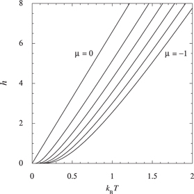
Figure 4. The temporal disorder of a bosonic gas in a single open channel of energy threshold  between r = 2 reservoirs characterized by the CNT entropy per unit time (62) in units of
  versus the thermal energy
  for the chemical potentials
  .
.
Download figure:
Standard image High-resolution imageFor bosons, the time-reversed coentropy per unit time is similarly given by

with the Bose–Einstein distribution  associated with the reservoir k of the incoming channel
  for the time reversal of the path
  . Consequently, we obtain

4.2. Thermodynamic entropy production
Here, the difference between the coentropy (64) and the entropy (62) per unit time takes the following form:

Since the Bose–Einstein distribution has the property

the difference is again given by equation (46). The energy and particle currents (47) and (48) can here also be identified. The Landauer–Büttiker formulas are recovered with the Bose–Einstein distributions. Therefore, equation (52) also holds for bosons so that the difference between the coentropy and entropy per unit time is again equal to the thermodynamic entropy production

as announced.
4.3. Full counting statistics and entropy production
For noninteracting bosons, Klich's formula

relates the many-body operators  and
and  to the corresponding one-body operators
  and
and  [57]. Using the same reasoning as for fermions, the cumulant generating function of all the bosonic currents reads

in terms of the scattering matrix  , the diagonal matrix
  formed with the Bose–Einstein distributions associated with every channel, and the diagonal matrices
  with the counting parameters
  . The multivariate exchange fluctuation theorem holds because the generating function (69) obeys the symmetry relation (34).
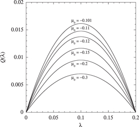
For bosons, the generating function has a similar shape as for fermions. This is illustrated in figure 5 for a single particle current across a delta barrier between two terminals. The chemical potentials of both reservoirs take negative values, as required by the condition  . The symmetry
  of the fluctuation theorem (34) with respect to the chemical affinity
  is confirmed.
Figure 5. The cumulant generating function  versus the counting parameter
  for the bosonic current across the delta barrier
  between two reservoirs at the chemical potentials
  with
with  and varying
  . The other parameter values are
  ,
,  , and
, and  . The transmission probability of the delta barrier is given by
  . The chemical affinity takes the value
  .
.
Download figure:
Standard image High-resolution image
The average values of the energy and particle currents deduced from the generating function are given by equations (55)–(56), which are equivalent to equations (47)–(48). Accordingly, the difference between the coentropy and the entropy per unit time is here also equal to the standard expression of the thermodynamic entropy production.
5. Conclusions
In this paper, a scattering approach to the thermodynamics of quantum transport is developed for noninteracting bosons or fermions in small open systems. This approach concerns the quantum transport of electrons in mesoscopic multiterminal circuits [31, 32, 35], as well as ultracold neutral atoms in optical traps with a tiny constriction separating two or more reservoirs at different chemical potentials or temperatures [33, 34]. The scattering approach is formulated in terms of the scattering matrix, which allows us to describe the quantum coherent dynamics of noninteracting bosons or fermions flowing across the open system.
The temporal disorder in the motion of bosons or fermions is characterized in terms of a dynamical entropy per unit time introduced in the eighties by CNT [24]. This CNT entropy per unit time is already positive for equilibrium many-body quantum systems at positive temperature such as gases of noninteracting bosons or fermions scattered in the constriction separating reservoirs at equal chemical potentials and temperatures. This confirms earlier results showing that classical or stochastic systems typically have a positive KS or  -entropy per unit time at equilibrium [10, 11, 63–69]. Contrary to the situation in stochastic systems where dynamical randomness exists down to arbitrarily small spatial or temporal scales leading to an infinite KS entropy per unit time, the CNT entropy per unit time remains bounded in quantum systems because there is no possible temporal disorder below the fundamental quantum limit given by Planck's constant on classically corresponding position-momentum or time-energy conjugated variables:
  or
or  .
.
In nonequilibrium steady states, the transport process is no longer symmetric under time reversal because the reservoirs have different chemical potentials or temperatures so that the forward and time-reversed histories have different probabilities. Therefore, the probabilities of the time reversals should decay with a rate different from the CNT entropy per unit time. This observation motivates the introduction of the time-reversed coentropy per unit time by averaging the decay rates of the probabilities of time-reversed histories over the typical forward histories. The result obtained in the present paper is that the difference between the coentropy and the CNT entropy per unit time is equal to the thermodynamic entropy production expressed as the sum of the thermal and chemical affinities multiplied by their corresponding mean energy and particle currents. This standard expression of entropy production is confirmed using the full counting statistics of bosons and fermions, for which the multivariate cumulant generating function of all the currents is deduced.
The relationships established in the present paper open new perspectives in the extension to quantum systems of results previously obtained for classical and stochastic systems. Since the scattering approach is not restricted to noninteracting particles, we may wonder if similar results could also be found for quantum many-body systems of interacting particles, which is a question left open for future investigations.
Acknowledgments
This research is financially supported by the Université Libre de Bruxelles and the Belgian Science Policy Office under the Interuniversity Attraction Pole project P7/18 'DYGEST'.