A nonlinear plasma retroreflector for single pulse Compton backscattering

Relativistic electrons counterpropagating with respect to a laser pulse undergo rapid oscillatory motion in the pulse's electromagnetic field. This motion results in the emission of photons that travel predominately in the direction of the relativistic electrons and possess frequencies twice Doppler upshifted from the pulse's frequency. The emission, referred to as Compton backscattering [1], has a frequency ω_C ∼ 4γ₀²ω₀, where ω₀ is the pulse frequency and γ₀ the electron relativistic factor. Thus depending on the electron energy and pulse frequency, the emitted radiation can range from extreme ultraviolet, ∼100 eV, to gamma, ∼1 MeV, energies. With such a broad range of frequencies, Compton backscattering has been proposed for several applications including, phase contrast imaging [2], radiosurgery [3], lithography [4], and nuclear resonance fluorescence [5].

Radio-frequency linacs produce high-energy, low emittance electron beams ideal for Compton backscattering [6, 7], but their size and cost are prohibitive for widespread deployment. All-optical Compton backscattering offers a potential small-scale alternative by replacing the linac with a laser wakefield accelerator. In a laser wakefield accelerator, the ponderomotive force of a high intensity, ultrashort laser pulse excites plasma waves whose fields can trap and accelerate electrons [8, 9]. Standard all-optical Compton scattering therefore requires two ultrashort laser pulses, one for driving the wakefield to inject and accelerate electrons and one for scattering [10]. While both pulses can be generated from the same laser by splitting the initial pulse and aligning the resultant pulses for counterpropagation, the process can be cumbersome.

Ta Phuoc et al demonstrated a single pulse scheme in which the wakefield driving pulse reflects from a self-generated plasma mirror at the surface of a CH or glass foil [11]. The reflected pulse then intersects the electrons trapped in the wakefield providing the wiggler. Solid foils have, however, limitations including erosion and bremsstrahlung emission from the accelerated electrons. Furthermore, the alignment issue is not completely eliminated: the pulse should intersect the foil at a small angle to ensure maximum overlap of the reflection and accelerated electrons.

Here we examine an alternative scheme for single ultrashort pulse Compton backscattering. The shaped gas target consists of two collinear gas jets. The first gas jet emits a light gas, helium for instance, while the second emits a heavier gas such as nitrogen. A long (nanosecond) pulse focused into the heavy gas jet launches a hydrodynamic shock wave that propagates toward the lighter gas. The shock wave and heavy gas jet flow collide forming a sharp density spike [12, 13] that eventually intersects the light gas.

The ultrashort laser pulse propagates from the light gas towards the density spike. The leading edge of the ultrashort laser pulse ionizes the light gas, while the bulk of the pulse drives a wakefield, accelerating electrons. As the short pulse intersects the density spike, its leading edge ionizes the heavy gas forming a plasma mirror. The bulk of the pulse undergoes a partial retroreflection from the mirror, providing a counterpropagating field. This field Compton backscatters from the wakefield accelerated electrons. A schematic of the interaction is displayed in figure 1.

Zoom In Zoom Out Reset image size

The major advantages of this scheme lie in the high rep-rate of the gas jet system and, as we will see, the significant retro-reflection of light from the spike. Furthermore, the long and short pulse lasers can be easily synchronized in experiments. The shock wave moves only a few microns in one nanosecond [12], while the density gradient at the shock wave spike is typically a few tens of microns long [13]. We note that depending on the heavy gas used, the long pulse may partially ionize the spike reducing the ionization burden of the short pulse. Additionally ultrashort laser prepulse or pedestal can be used for gas ionization. Such pedestals can be generated in a controlled manner by the manipulation of the laser system bandwidth [14].

Optimizing the Compton radiation requires characterization of the counterpropagating field and an understanding of the mechanisms responsible for the retroreflection. Using the full format particle-in-cell (PIC) simulation TurboWAVE [15], we investigate the Poynting flux reversal and resulting Compton spectrum as a function of incident pulse amplitude and plasma spike profile. We identify two physical processes responsible for the nonlinear retroreflection from the plasma mirror: saturation of the absolute Raman instability at the quarter critical surface and Bragg-like reflections from a nonlinear density fluctuation formed near the critical surface. To our knowledge, we are the first to demonstrate the role of these processes in high-intensity, ultrashort pulse reflections from plasma mirrors. We describe these mechanisms in more detail below.

For normal incidence, we simply refer to the reversal as a reflection. In this case we find that there are two regimes depending on the density of the spike. For low spike densities n_sp < n_cr, where n_cr = m_eω₀²/4πe² is the critical density, the reflection occurs predominately at the quarter critical surface, resulting in a backscattered spectrum centered near ω₀/2. This reflection is a general phenomenon occurring when high intensity light interacts with a quarter critical surface [16–19]. Previous studies, however, were motivated by laser-based inertial confinement fusion and thus characterized by low intensity, $I\lt {{10}^{17}}\;{\rm W}\;{\rm c}{{{\rm m}}^{-{\rm 2}}},$ long pulses, τ > 10 ps, and hot plasmas, ${{T}_{{\rm e}}}\gt 500\;{\rm eV}.$ More recent observations of these reflections have been made in the context of highly oblique angle ultrashort pulse–solid interactions for electron heating [20, 21]. Our interest here is in high intensity $I\gt 5\times {{10}^{17}}\;{\rm W}\;{\rm c}{{{\rm m}}^{-{\rm 2}}},$ ultrashort pulses, τ ≤ 50 fs in cold plasmas. We make the connection between this reflection and the saturation of the absolutely unstable Raman instability [16], which by itself would only allow stationary scattering. Bonnaud et al suggested a similar mechanism for long pulses, in which the absolute Raman instability seeds the backscattered convective wave [19].

Most of the incident pulse energy makes it past the quarter critical layer. For higher spike densities n_sp ∼ n_cr, a second, more efficient reflection occurs as the result of a spatially periodic electron density fluctuation that develops near the critical surface. The ponderomotive force generated by the spatial overlap of the reflected and incident pulse drive the electron density fluctuation. The density fluctuation modifies the local plasma dielectric constant, providing a Bragg-like grating that enhances the reflection. The resulting reflected spectrum is centered near ω₀.

We also show that the properties of the Compton x-ray spectrum are determined primarily by the amplitude of the incident pulse and are relatively insensitive to the spike density. For instance, if the incident pulse amplitude is low, a₀ = 0.5, the reflected pulse provides a narrow band x-ray spectrum characteristic of small amplitude Compton scattering [22]. If, on the other hand, the incident pulse amplitude is large, a₀ > 1.0, the reflected pulse is nonlinear, providing a broadband Compton x-ray spectrum [22]. Finally, we find that for non-normal incidence of the pulse, a significant fraction of energy is reflected directly backward, ensuring the robustness of our scheme to small alignment errors. Specifically, the insensitivity of the Compton x-ray spectrum is demonstrated for incidence angles between 1° and 5°.

The remainder of the manuscript is organized as follows. Section 2 details the set up for our simulations. In section 3 we present simulation results for pulses normally incident on the density spike and explain the mechanisms behind the nonlinear reflection. This includes a discussion of 3D effects. In section 4 we present the Compton spectra resulting from normally incident pulses and discuss the effects leading to the spectral features. Section 5 includes our results for the nonlinear reflection and Compton scattering from pulses non-normally incident on the density spike. Section 6 concludes the paper with a summary of our results.

To investigate the laser pulse–density spike interaction we conducted PIC simulations using TurboWAVE [15]. TurboWAVE is a framework for solving the Maxwell–Lorentz system of equations for charged particle dynamics. The model is fully relativistic and fully electromagnetic. The fields are advanced with a Yee solver [23], and the sources are deposited using quadratic weighting, with charge conservation ensured by means of a Poisson solver.

The fields, particle trajectories, densities, and currents were calculated on a 2D or 3D planar-Cartesian grid in the lab frame. The 3D simulation domain was 183 × 183 × 214 μm in the transverse, $x$ and $y,$ and longitudinal directions, $z,$ respectively. For the 2D simulations the $y$ direction was eliminated. The cell sizes were chosen to resolve the laser wavelength along the propagation direction. The specific values will be presented with each case. The relatively short axial domain was motivated by computational considerations. Because our interest lies in the properties of the reflected light, the simulations must be conducted in the lab frame as opposed to the moving frame. This places a higher computational cost on the total simulated distance, which can be mitigated by considering a shorter axial domain. We discuss the physical ramifications of this below.

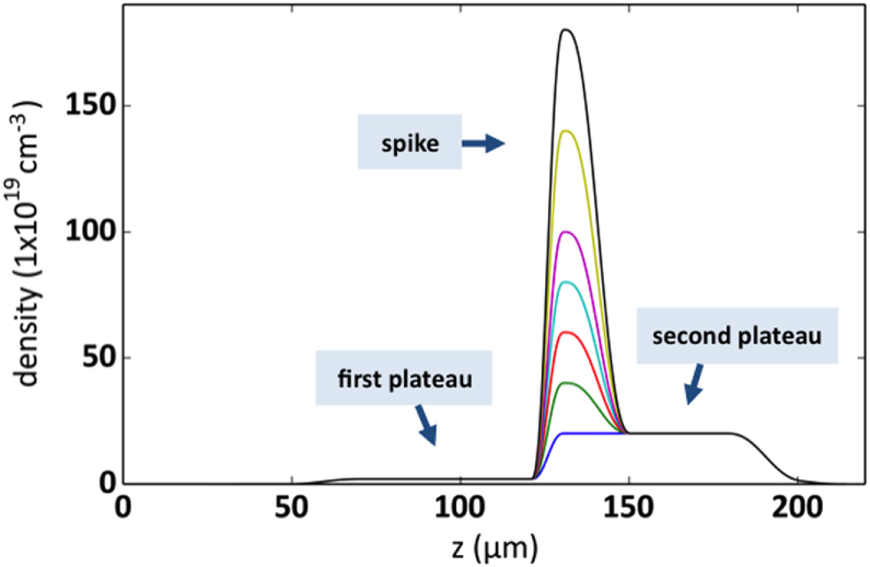
The plasma density profile was chosen to represent the intersection of a hydrodynamic shock launched in a heavy gas with a low density, light gas region. In the simulation, the gas was pre-ionized, and the ions were immobile providing only a neutralizing background. The electron density initially ramped up over 24 μm to a density of 2 × 10¹⁹ cm⁻³. Following a plateau of 50 μm, the electron density again ramped up over 10 μm to peak density, which was varied between 2 × 10²⁰ and 1.8 × 10²¹ cm⁻³. After the peak, the density returned, over 20 μm, to a value of 2 × 10²⁰ cm⁻³ where it remained until a final down ramp of 24 μm. The simulated density profiles are illustrated in figure 2.

Zoom In Zoom Out Reset image size

The laser pulse was initialized with x linear polarization, a sin² temporal profile, and a Gaussian transverse profile. The pulse parameters were as follows: central wavelength λ = 800 nm, temporal full width half maximum (FWHM) τ = 50 fs, and an ${\rm exp} (-1)$ field width w = 23 μm. The normalized field amplitude, ${{a}_{0}}=eE/{{m}_{{\rm e}}}c{{\omega }_{0}},$ where ${{\omega }_{0}}=2\pi c/\lambda ,$ m_e is the electron mass, c the speed of light, and e the fundamental unit of charge, was varied between 0.5 and 2.0. These parameters correspond to pulse energies between 0.22 and 3.5 J. The pulse started with its front edge at the beginning of the density ramp and centered along the z-axis. To change the laser pulse's angle of incidence with respect to the spike, the spike profile was rotated in the x–z plane, while keeping the propagation axis aligned with the z-axis.

In practice, the length of the first plateau would be determined by the desired electron energy for Compton scattering. Depending on the plateau length, the pulse profile may evolve as it propagates to the density spike. For laser wakefield acceleration (LWFA) the primary evolution mechanisms are diffraction, self-focusing, and pulse energy depletion. In both the linear $({{a}_{0}}\ll 1)$ and nonlinear regimes $({{a}_{0}}\gg 1)$ of matched LWFA, the depletion length is greater than or equal to the dephasing length, the length over which electrons outrun the accelerating phase of the wakefield [24]. As a result, significant pulse evolution through depletion typically occurs after the maximum electron energy gain [25]. For all ${{a}_{0}}$ considered here the power exceeds the critical power for self-focusing: $P/{{P}_{c}}={{\left( {{k}_{{\rm p}}}w \right)}^{2}}a_{0}^{2}/32{\mkern 1mu} \gt {\mkern 1mu} 1,$ abating diffraction. Furthermore, self-focusing can preserve a Gaussian-like transverse profile [26] such that the simulated pulses can be considered representative of pulses having been self-focusing from the start of a longer plateau.

We begin by considering the reflection of normally incident p-polarized laser pulses from spikes of varying density. We conducted a single 3D simulation to verify the phenomena observed in 2D simulations, which we present later in this section. The 3D simulation domain was discretized with 256 × 256 × 8192 cells in the transverse, $x$ and $y,$ and longitudinal directions, $z,$ respectively. Figure 3 illustrates the 3D transmission and reflection of an a₀ = 1.0 pulse from a spike of density 1 × 10²¹ cm⁻³ or 0.57 n_cr, where ${{n}_{{\rm cr}}}={{m}_{{\rm e}}}\omega _{0}^{2}/4\pi {{e}^{2}}=1.7\times {{10}^{21}}\;{\rm c}{{{\rm m}}^{-3}}$ is the critical density. The figure displays snapshots of the pulse intensity envelope before during and after the reflection at t = 280 fs, t = 340 fs, t = 400 fs, and t = 460 fs. In each frame, the incident or transmitted pulse propagates from the lower right to the upper left. At 400 fs the reflected and transmitted pulses have spatially separated. The reflected pulse emanates from the center of the incident pulse resulting in the centralized intensity depletion in the transmitted pulse by 460 fs. Surprisingly, the reflected pulse's peak intensity is comparable to that of the incident pulse. The local depletion and reflection demonstrate nonlinearity: the reflected and transmitted energy depend on the local intensity of the incident pulse. The major difference between the 3D and 2D results was in the intensity of the reflected pulse. Nonlinear focusing in the high-density plasma led to a 1.5x enhancement in the peak reflected intensity in 3D. Other than the intensity enhancement, the spatial profiles in both 2D and 3D were quite similar.

Zoom In Zoom Out Reset image size

We continue by considering 2D simulations, which allow investigation of a wider parameter range. This is particularly useful for optimizing the reflected pulse for Compton backscattering. For the following results, the simulation domain was discretized with 256 × 16 384 cells. Once the transmitted and reflected pulses become spatially distinct, we can calculate the fraction of energy reflected and transmitted by integrating over the region of space containing each pulse. In particular we define the reflection fraction, $R,$ and transmission fraction, $T,$ as

$$\begin{eqnarray}&&R=\frac{1}{4\pi {{U}_{{\rm L}}}}\int {{{\rm d}}^{2}}{{{\bf x}}_{\bot }}\int \limits_{0}^{{{z}_{{\rm S}}}-\Delta } {{{\bf E}}^{2}}{\rm d}z,\end{eqnarray} \tag{ 1a }$$

$$\begin{eqnarray}&&T=\frac{1}{4\pi {{U}_{{\rm L}}}}\int {{{\rm d}}^{2}}{{{\bf x}}_{\bot }}\int \limits_{{{z}_{{\rm S}}}+\Delta }^{{{z}_{{\rm max} }}} {{{\bf E}}^{2}}{\rm d}z,\end{eqnarray} \tag{ 1b }$$

where ${{z}_{{\rm S}}}$ marks the peak of the spike, $\Delta$ is the width of the spike, ${{z}_{{\rm max} }}$ is the axial simulation boundary, and ${{U}_{{\rm L}}}$ is the incident laser pulse energy. The use of $\Delta$ eliminates electrostatic energy contributions within the spike, which along with the plasma kinetic energy account for the absorbed pulse energy. In equation (1) we have approximated the total electromagnetic energy density by twice the contribution from the electric field. We have verified that the electrostatic contribution to $R$ and $T$ outside of the spike is small in regions devoid of the pulse (less than 1% of the energy density localized in the spike). From equation (1) we can also obtain the absorption fraction: $A=1-R-T$.

Figure 4 displays the reflection and absorption fractions as a function of peak spike density. The general trends are that $R$ increases with electron density, and $A$ increases with a₀. From a₀ = 1.0 to a₀ = 2.0, the increase in $A$ coincides with the drop in $R.$ We note that, in general, the peak reflected amplitude, ${{a}_{{\rm R}}},$ is greater than ${{R}^{1/2}}{{a}_{0}}.$ Several effects contribute to the sharp increase in reflected and absorption fractions for a₀ > 0.5. Foremost, we have already seen in figure 3 that the reflection is nonlinear. The area of the pulse that can drive the nonlinearity and, as a result, be depleted increases with a₀. To understand the other contributing effects and nonlinearity in more detail, we turn to figure 5. Figure 5 shows the spatial power spectral density (PSD) of the reflected pulse for each incident a₀ and n_sp. The red dashed and solid lines mark k = k₀ and k = k₀/2 respectively, and each PSD curve has been normalized to its maximum. The ${{n}_{{\rm sp}}}=2\times {{10}^{20}}\;{\rm c}{{{\rm m}}^{-{\rm 3}}}$ curve for ${{a}_{0}}=0.5$ has been omitted because the reflected energy was nearly zero. For each incident pulse amplitude, the PSD exhibits two qualitative behaviors depending on the spike density. At low spike densities, 4 × 10²⁰ cm⁻³ < n_sp ≤ 1.0 × 10²¹ cm⁻³, the spectral peak occurs near k₀/2, while at higher densities, n_sp ≥ 1.4 × 10²¹ cm⁻³, the peak is shifted towards k = k₀.

Zoom In Zoom Out Reset image size

Zoom In Zoom Out Reset image size

At the lower spike densities the reflection results from the saturation of the absolute Raman backscattering instability. Near the quarter critical density, n_cr/4 ∼ 4 × 10²⁰ cm⁻³, the incident electromagnetic pulse undergoes resonant Raman scattering and decays into a scattered electromagnetic and electrostatic wave each with a frequency ω_s ∼ ω₀/2 ∼ ω_p. The scattering is absolutely unstable and both scattered waves are trapped in a region near the quarter critical surface where they undergo temporal growth [16]. Drake and Lee have analyzed the instability in detail [16]. In their analysis, the parameter $N={{2}^{-1/2}}a_{0}^{3/2}{{k}_{0}}L$ quantifies the strength of the inhomogeneity, where $L$ is the gradient scale length at the quarter critical surface, $L\sim \left[ {{\partial }_{z}}{\rm ln} \left( {{n}_{{\rm e}}} \right) \right]{{|}_{z={{z}_{{\rm qc}}}}},$ and ${{z}_{{\rm qc}}}$ is the axial position of the surface. Values of $N\gg 1$ and $N\ll 1$ indicate weak and strong imhomogeneity respectively. The lower spike densities, n_sp < 1.4 × 10²¹ cm⁻³, have scale lengths $L\gt 2.4\;\mu {\rm m},$ and thus $N\gt 5$ for each a₀ we consider. Even though the gradients are comparable to the laser wavelength, the relatively large amplitudes place our parameters well within the weakly inhomogeneous regime.

For weak inhomogeneity, the temporal growth rate, Γ, scattered frequency of the electromagnetic wave, ω_EM, and total width of the absolutely unstable region, δz, are given by the following:

$$\begin{eqnarray}&&\frac{\Gamma }{{{\omega }_{{\rm pq}}}}\cong \frac{\sqrt{3}}{2}{{a}_{0}}\left[ 1-{{\left( \frac{1}{12} \right)}^{1/4}}{{N}^{-1}} \right],\end{eqnarray} \tag{ 2a }$$

$$\begin{eqnarray}&&\frac{{{\omega }_{{\rm EM}}}}{{{\omega }_{{\rm pq}}}}\cong \left[ 1{\mkern 1mu} +{\mkern 1mu} 4\sqrt{3}{{\left( \frac{{{\omega }_{{\rm pq}}}}{\Gamma } \right)}^{1/2}}{{N}^{-5}} \right],\end{eqnarray} \tag{ 2b }$$

$$\begin{eqnarray}&&\begin{array}{lllllllllllllll} {{k}_{{\rm pq}}}\delta z={{\left( \frac{3}{2} \right)}^{1/2}}a_{0}^{-1/2}N\left( \frac{{{k}_{{\rm pq}}}}{{{k}_{0}}} \right) \\ \quad \quad \quad \;\times {{\left[ 1-\frac{4}{3}a_{0}^{-2}{{\left( \frac{\Gamma }{{{\omega }_{{\rm pq}}}} \right)}^{2}} \right]}^{1/2}}, \\ \end{array}\end{eqnarray} \tag{ 2c }$$

where $\omega _{{\rm pq}}^{2}=\pi {{e}^{2}}{{n}_{{\rm cr}}}/{{m}_{{\rm e}}}$ is the plasma frequency at the quarter critical surface. To estimate the effect of relativistic pump amplitudes, we can apply to equation (2) the transformations $\omega _{{\rm pq}}^{2}\to {{\gamma }_{\bot }}\omega _{{\rm pq}}^{2}$ and ${{a}_{0}}\to {{a}_{0}}/\gamma _{\bot }^{1/2},$ where ${{\gamma }_{\bot }}={{\left( 1+a_{0}^{2}/2 \right)}^{1/2}}$ is the relativistic factor accounting the electron's rapid motion in the pump field. Figure 4 indicates a density dependence of the reflected and absorbed energy fraction, but Γ and ω_EM in equation (2) only depend weakly on density through $N$ by way of $L.$ So where then does the density dependence of figure 4 originate? The local group velocity of the incident pulse can be written ${{v}_{g0}}(z)/c\sim 1-\omega _{{\rm p}}^{2}(z)/2\omega _{0}^{2}.$ In a sharp, increasing density gradient, the group velocity at the back of the pulse is larger than that in the front. This results in a compression of the pulse or 'swelling' that increases the pulse amplitude. Assuming fixed energy and a flat-top temporal pulse shape, one can show that the amplitude increases as ${{a}_{{\rm sw}}}(z)\sim {{a}_{0}}{\rm exp} \left[ \left( \omega _{{\rm pq}}^{2}/4\omega _{0}^{2} \right)(z/L) \right].$ Taking z = 5 μm we find ${{a}_{{\rm sw}}}/{{a}_{0}}~\sim ~1.07,$ 1.11, and 1.14 for n_sp = 6.0, 8.0, and 10.0 × 10²⁰ cm⁻³ respectively. These small changes in the pulse amplitude increase ${\rm exp} (\Gamma \tau )$ substantially.

Equation (2) and the swelling model illustrate three points. First, the growth rate of the instability and hence the reflected and absorbed energy increase with both a₀ and ${{n}_{{\rm sp}}}$ consistent with figure 4. As an example, using a spike density n_sp = 1.0 × 10²¹ cm⁻³, the incident pulse FWHM as the exponentiation time, and the simple estimate of compression, the gains are Γτ ∼ 22, 50, and 100 for a₀ = 0.5, 1.0, and 2.0 respectively. Second, the frequency of the scattered electromagnetic wave is nearly ${{\omega }_{{\rm pq}}}$ consistent with figure 5. Finally, the absolute instability is localized to a region of ∼7 μm. The absolute Raman theory also explains the reduced downshifting of the spectral peak for a spike density of n_sp = 2 × 10²⁰ cm⁻³ < n_cr/4 and amplitudes a₀ ≥ 1.0 in figure 5.

The analysis of Drake and Lee [16] provides a framework to understand the reflection, but their treatment is limited to a non-evolving continuous, plane pump wave and the linear stage of instability. For examining non-ideal effects, we return now to the simulations. Figure 6 displays contributions to the electromagnetic energy density from different spectral ranges and field components as a function of time and axial coordinate. The incident pulse amplitude and spike density are a₀ = 0.5 and n_sp = 1 × 10²¹ cm⁻³ respectively. The contributions have been averaged over the transverse coordinate and normalized to their peak values for clarity. The dashed white line marks the quarter critical surface. In figure 6(a) the energy density of the incident pulse is plotted. The contours have a positive slope representing forward propagation. The drop off in energy density occurs due to the reduction in wavenumber as the plasma density increases: for fixed frequency $c{{k}_{z}}\sim {{\left[ {{\omega }^{2}}-\omega _{{\rm p}}^{2}(z)-{{c}^{2}}k_{\bot }^{2} \right]}^{1/2}}.$ In figure 6(b) we see the electrostatic energy density initially grow in time and remain stationary (non-convecting) at the quarter critical surface. Figure 6(c) shows the stationary, near zero wavenumber, localized growth, of the electromagnetic energy at the quarter critical surface. These first three subplots illustrate the expected energetics of the three waves interacting in the absolute Raman instability.

Zoom In Zoom Out Reset image size

We have yet to explain why an absolute instability leads to the emission of a convecting electromagnetic wave, aka our reflected pulse. In both figures 6(b) and (c) we see the energy density grow rapidly in time and then abruptly crash (the electrostatic energy density goes through several such cycles). The emission of the reflected pulse occurs simultaneously with this crash as can be seen in figure 6(d) where the reflected pulse appears as the negative slope contours. Thus we conclude that the reflected pulse results from the absolute Raman instability's saturation. The seeding of the convective wave by the absolute Raman instability has also been suggested in the context of low-intensity, long pulse–quarter critical interactions [19]. One could also put forth the explanation that the trapping 'potential' disappears as the incident pulse convects away from the quarter critical region. However, figure 6 shows that the incident pulse is still within this region.

The dynamics are similar for larger amplitudes, a₀ = 1.0 to a₀ = 2.0, but the growth, saturation, and emission cycles can occur several times. Nonlinear evolution of the incident wave, including depletion and spectral broadening, introduces additional complexity. In spite of this, a simple explanation can be offered for the broad spectra redshifted beyond k₀/2 observed in figure 5. The reflected pulse originates in a high-density region possessing a wavelength twice that of the pump and an amplitude nearly as large. Each of these, the high density, long wavelength, and high amplitude, make the reflected pulse itself susceptible to Raman instabilities. For instance, as the reflected pulse propagates into lower densities, it encounters its own quarter critical surface where it undergoes absolutely unstable Raman scattering, while at slightly lower densities it undergoes Raman forward scattering [27, 28]. This additional nonlinear scattering leads to the complicated spectra at lower spike densities, 4 × 10²⁰ cm⁻³ < n_sp ≤ 1.0 × 10²¹ cm⁻³, for a₀ = 1.0 and a₀ = 2.0.

The incident pulse retains much of its energy after interacting with the initial critical surface: more than 95% for the parameters considered in figure 6. For lower spike densities, n_sp ≤ 1.4 × 10²¹ cm⁻³, what remains of the incident pulse interacts with the quarter critical surface at the back of the spike before propagating away. For larger spike densities, the leading edge of the pulse undergoes a partial reflection from the near critical density surface. The ponderomotive force generated by the spatial overlap of the pulse and its reflection sets up a stationary periodic density fluctuation: $\delta n\sim {\rm cos} \left( {{k}_{0}}z-{{\omega }_{0}}t \right){\rm cos} \left( {{k}_{0}}z+{{\omega }_{0}}t \right)$ or $\delta n\sim {\rm cos} \left( 2{{k}_{0}}z \right).$ This density fluctuation, δn, when added to the background electron density can exceed the critical density, ${{n}_{0}}+\delta n\gt {{n}_{{\rm cr}}},$ where n₀ is the local electron density, while the periodicity provides a Bragg-like grating. An ideal Bragg grating consists of alternating layers of materials with different dielectric constants. The light incident on each interface contributes a Fresnel (linear) reflection that can add constructively with the reflections from all other interfaces, leading to a reflection far surpassing that of a single dielectric slab. Here the spatial oscillations in electron density act as the alternating layers.

Figure 7 displays the on-axis intensity, calculated from $E_{x}^{2},$ (right scale, blue) and absolute electron density fluctuation (left scale, red) enveloped at the incident pulse wavenumber as a function of axial coordinate at 337 fs. The incident pulse amplitude and peak spike density are a₀ = 1.0 and n_sp = 1.4 × 10²¹ cm⁻³ respectively. The left dashed black line marks the quarter critical surface, and the right dashed black line the location of the peak spike density. The figure demonstrates the large periodic electron density fluctuation set up by the ponderomotive force of the incident and reflected light. As seen in figure 4, the reflection fraction is relatively large for a₀ = 1.0 and 2.0 when n_sp = 1.4 × 10²¹ cm⁻³ in spite of the background electron density being lower than the critical density. This is a direct result of the large density fluctuation acting as a Bragg-like mirror. Additionally, the weak reflection of a₀ = 0.5 when n_sp = 1.4 × 10²¹ cm⁻³ results from the pulse amplitude being too small to set up a large density fluctuation.

Zoom In Zoom Out Reset image size

As a comparison, we consider the reflection fraction from a single dielectric slab predicted by Fresnel theory:

$$\begin{eqnarray}&&{{R}_{{\rm F}}}=\frac{\eta _{{\rm L}}^{2}+\eta _{{\rm R}}^{2}+2{{\eta }_{{\rm L}}}{{\eta }_{{\rm R}}}{\rm cos} \left( 2{{k}_{{\rm S}}}\Delta \right)}{1+\eta _{{\rm L}}^{2}\eta _{{\rm R}}^{2}+2{{\eta }_{{\rm L}}}{{\eta }_{{\rm R}}}{\rm cos} \left( 2{{k}_{{\rm S}}}\Delta \right)},\end{eqnarray} \tag{ 3 }$$

where ${{\eta }_{{\rm L}}}=\left( \varepsilon _{{\rm S}}^{1/2}-\varepsilon _{{\rm L}}^{1/2} \right)/\left( \varepsilon _{{\rm S}}^{1/2}+\varepsilon _{{\rm L}}^{1/2} \right),$ ${{\eta }_{{\rm R}}}=\left( \varepsilon _{{\rm R}}^{1/2}-\varepsilon _{{\rm S}}^{1/2} \right)/\left( \varepsilon _{{\rm R}}^{1/2}+\varepsilon _{{\rm S}}^{1/2} \right),$ ${{\varepsilon }_{x}}=1-\omega _{{\rm p}x}^{2}/\omega _{0}^{2}$ is the dielectric function of the plasma, and L, S, and R denote the regions left of the spike, the spike itself, and right of the spike. For n_sp = 1.4 × 10²¹ cm⁻³, upon taking Δ = 9 μm and setting ${{k}_{{\rm S}}}=\varepsilon _{{\rm S}}^{1/2}{{\omega }_{{\rm S}}}/c,$ equation (3) predicts ${{R}_{{\rm F}}}=0.07.$ This is comparable to the value calculated by equation (1a) for a₀ = 0.5, $R=0.03,$ but much smaller than the value for a₀ = 1.0, $R=0.35.$ The disagreement cannot be explained by including the effect of relativistic transparency through the transformation $\omega _{{\rm p}}^{2}\to \omega _{{\rm p}}^{2}/{{\gamma }_{\bot }}$ in equation (3). In fact, this transformation makes the disagreement with a₀ = 1.0 even worse. Furthermore, equation (3) is sensitive to Δ: it predicts small reflection fractions over limited ranges of Δ, while the reflections we observe are quite robust.

However, as discussed above, the a₀ = 1.0 pulse drives a periodic density fluctuation resulting in a total electron density, ${{n}_{{\rm sp}}}+\delta n,$ sufficient to set up a Bragg mirror that enhances the reflection. For an ideal Bragg grating the reflection fraction is given by

$$\begin{eqnarray}&&{{R}_{{\rm B}}}={{\left| \frac{\kappa {\rm sinh} (\Gamma \ell )}{\Gamma {\rm sinh} (\Gamma \ell )-{\rm i}\delta {\rm sinh} (\Gamma \ell )} \right|}^{2}},\end{eqnarray} \tag{ 4 }$$

where $\Gamma ={{\left( {{\kappa }^{2}}-{{\delta }^{2}} \right)}^{1/2}},$ $\kappa =\left( {{k}_{0}}/\pi \right)\left( \varepsilon _{{\rm max} }^{1/2}-\varepsilon _{{\rm min} }^{1/2} \right),$ $\delta =\left\langle {{\varepsilon }^{1/2}} \right\rangle {{k}_{0}}-\pi /{{\lambda }_{{\rm B}}},$ $\left\langle {{\varepsilon }^{1/2}} \right\rangle$ is the average refractive index in the grating, ${{\lambda }_{{\rm B}}}$ is the periodicity of the grating, and $\ell$ is the total length of the grating [29]. Using figure 7 as an example, we set δn = 1 × 10²⁰ cm⁻³, ${{\lambda }_{{\rm B}}}=800\;{\rm nm}$ , and $\ell =4\;{\rm mm}$ and find R_B = 0.42. This reflection fraction is comparable but greater than that observed in figure 4. A small disagreement, however, is not surprising: the ideal analysis neglects the changes in $\delta n$ along the spike, the transmission of light through the back of the spike, and absorption. The Bragg-mirror picture also explains the limited reflection for a₀ = 0.5. The ponderomotive force when a₀ = 0.5 is too weak to generate a δn large enough for reflection.

In support of a Bragg-like reflection, we observe smaller shifts in the wavenumber of the reflected pulse than in the absolute Raman mechanism. This can be observed in figure 5. When a₀ = 0.5 and a₀ = 1.0 with n_sp = 1.4 × 10²¹ cm⁻³, spectral signatures are present at k₀/2 and k₀ corresponding to the reflections from the quarter critical and near-critical density surfaces respectively. Again the complicated spectral structure for a₀ = 1.0 and a₀ = 2.0 can be explained by additional Raman scattering of the reflected wave as it propagates out of the spike region.

In our scheme, the reflected pulse Compton backscatters from electrons accelerated in the wakefield driven by the incident pulse. The bandwidth, amplitude, and direction of the reflected pulse will determine the bandwidth and energy fluence of the Compton x-rays. For instance, a narrow band, low amplitude scattering pulse will result in a narrow band x-ray spectrum with low fluence, while a broadband, high amplitude scattering pulse will result in a broadband spectrum with high fluence. The connection between the pulse and x-ray spectrum is made through the trajectories of the relativistic electrons. Esarey et al derived expressions for the trajectories of relativistic electrons counterpropagating with respect to an optical field. In their treatment, the optical pulse depends only on the moving frame coordinate $\xi =z+ct,$ and finite pulse duration and diffraction effects are ignored [22, 30]. As seen in figure 3 it is not clear that these assumptions are valid for our reflected pulses. We will refer to the trajectories and resulting Compton spectra of Esarey et al as the ideal case.

In particular, upon adapting their results for our reflected pulse, we have

$$\begin{eqnarray}&&x={{x}_{0}}+\frac{{{a}_{{\rm R}}}}{\left( 1+{{\beta }_{0}} \right){{\gamma }_{0}}{{k}_{{\rm R}}}}{\rm sin} \left( {{k}_{{\rm R}}}\xi \right),\end{eqnarray} \tag{ 5a }$$

$$\begin{eqnarray}&&\begin{array}{lllllllllllllll} z={{z}_{0}}+\frac{1}{2}\left[ 1-\frac{\gamma _{\bot }^{2}}{\gamma _{0}^{2}{{\left( 1+{{\beta }_{0}} \right)}^{2}}} \right]\xi \\ \quad \;\;-\frac{a_{{\rm R}}^{2}}{8\gamma _{0}^{2}{{\left( 1+{{\beta }_{0}} \right)}^{2}}{{k}_{{\rm R}}}}{\rm sin} \left( 2{{k}_{{\rm R}}}\xi \right), \\ \end{array}\end{eqnarray} \tag{ 5b }$$

where a_R and ${{k}_{{\rm R}}}$ are the amplitude and wavenumber of the reflected light respectively, ${{\gamma }_{0}}={{\left( 1-\beta _{0}^{2} \right)}^{-1/2}}$and, ${{\beta }_{0}}={{v}_{z0}}/c$ is the initial normalized electron velocity. With the analytic trajectories, the radiated spectrum can be calculated from

$$\begin{eqnarray}&&\frac{{{{\rm d}}^{2}}U}{{\rm d}\omega {\rm d}\Omega }=\frac{{{e}^{2}}{{\omega }^{2}}}{4{{\pi }^{2}}c}{{\left| \int {\rm d}t\left[ {\bf n}\times ({\bf n}\times {\boldsymbol{ \beta }} ) \right]{\rm exp} \left[ {\rm i}\omega \left( t-{\bf n}\cdot {\bf x}/c \right) \right] \right|}^{2}},\end{eqnarray} \tag{ 6 }$$

where Ω is the solid angle, β = v/c is the normalized electron velocity, and n is the unit vector pointing to the location of observation [31]. Esarey et al evaluate equation (6) in the limit a_R ≪ 1 and a_R ≫ 1. In the low amplitude limit, equation (6) evaluated in the forward direction is given by

$$\begin{eqnarray}&&{{\left. \frac{{{{\rm d}}^{2}}U}{{\rm d}\omega {\rm d}\Omega } \right|}_{\theta =0}}=\frac{{{e}^{2}}}{8\pi c}a_{{\rm R}}^{2}\left( {{k}_{{\rm R}}}{{L}_{\operatorname{int}}} \right)\left( \frac{{{\omega }_{C}}}{{{\omega }_{{\rm R}}}} \right){{\omega }_{C}}\delta \left( \omega -{{\omega }_{C}} \right),\end{eqnarray} \tag{ 7a }$$

while in the high amplitude limit

$$\begin{eqnarray}&&{{\left. \frac{{{{\rm d}}^{2}}U}{{\rm d}\omega {\rm d}\Omega } \right|}_{\theta =0}}=\frac{6}{{{\pi }^{3}}}\frac{{{e}^{2}}}{c}\left( {{k}_{{\rm R}}}{{L}_{\operatorname{int}}} \right)\gamma _{0}^{2}{{\left( \frac{\omega }{{{\omega }_{K}}} \right)}^{2}}K_{2/3}^{2}\left( \frac{\omega }{{{\omega }_{K}}} \right),\end{eqnarray} \tag{ 7b }$$

where ${{L}_{\operatorname{int}}}$ is the interaction distance of the reflected pulse and relativistic electrons, half the reflected pulse duration for instance, ${{\omega }_{K}}=3a_{{\rm R}}^{3}\gamma _{0}^{2}/\left( 1+a_{{\rm R}}^{2}/2 \right),$ and $K$ is the modified Bessel function. Equation (7) shows that, in the ideal case, a low amplitude pulse results in a narrow x-ray spectrum centered about ${{\omega }_{C}}=4a_{{\rm R}}^{2}\gamma _{0}^{2},$ while a high amplitude pulse results in a broad spectrum with characteristic width ${{\omega }_{K}}.$ This is precisely what we observe in the simulations.

Figure 8 displays single particle Compton radiated spectra in the forward, positive z direction, resulting from reflections of incident pulses with a₀ = 0.5, a₀ = 1.0, and a₀ = 2.0 and spike densities n_sp = 1.0 × 10²¹ cm⁻³ and n_sp = 1.8 × 10²¹ cm⁻³. The frequency is normalized to 4γ₀²ω₀. The spectra were calculated from equation (6) using trajectories of test particles with γ₀ = 19.6 started on-axis, 22 μm behind the peak of the laser pulse and evolved in the self-consistent fields of the simulation. Spectra were also calculated for initial energies of γ₀ = 98.0, 196, 391, and 978, but are not shown because the spectral features were nearly identical. We note that due to the short simulation distance, the test electrons were not accelerated in the pulse's wakefield and were meant to be representative of wakefield accelerated electrons. The densities were chosen such that scattering pulses were representative of reflections from the quarter critical surface and the critical surface. In each case, the peak amplitude of the reflected pulse was comparable to that of the incident pulse.

Zoom In Zoom Out Reset image size

The a₀ = 0.5 pulse results in a narrow band spectrum for both densities with peaks at ω/4γ₀²ω_R ∼ 1, where ω_R = ck_R: ω_R = ω₀/2 or ω₀ for n_sp = 1.0 × 10²¹ cm⁻³ or n_sp = 1.8 × 10²¹ cm⁻³ respectively. Interestingly, at n_sp = 1.8 × 10²¹ cm⁻³ the Compton spectrum exhibits a signature of the pulse reflection at n_c/4 as a tail extending from ω = 1 to 1/2. For both a₀ = 1.0 and a₀ = 2.0, the gross spectrum is broad but is not a smooth curve as predicted by equation (7b). This results from not being in the asymptotic limit of a_R ≫ 1.0, the finite temporal limits of integration in equation (6), and finite pulse duration effects such as the electron interacting with a range of amplitudes. The a₀ = 1.0 and a₀ = 2.0 pulse result in more total energy: when n_sp = 1.8 × 10²¹ cm⁻³, dU/dΩ = 26 and 40 keV compared to 6 keV for a₀ = 0.5.

The incoherence of the reflected field can also result in non-ideal electron motion, which can potentially modify the spectral properties of the Compton radiation. The degree of spatial coherence for the transverse component of the reflected field, ${{E}_{{\rm W}}}={\bf \hat{x}}\cdot {{{\bf E}}_{{\rm R}}}$ (wiggler field) evaluated on-axis is given by

$$\begin{eqnarray}&&G(z)=\frac{\int {{E}_{{\rm W}}}(z^{\prime} ){{E}_{{\rm W}}}(z^{\prime} -z){\rm d}z^{\prime} }{\int E_{{\rm W}}^{2}(z^{\prime} ){\rm d}z^{\prime} },\end{eqnarray} \tag{ 8 }$$

with the associated coherence length ${{\ell }_{z}}=\int {{\left| {\mkern 1mu} G(z) \right|}^{2}}{\rm d}z.$ For a₀ = 0.5, 1.0, and 2.0 respectively we find ${{\ell }_{z}}~=~16,$ 15, and 12 μm respectively. While the wiggler field coherence length is similar for a₀ = 0.5 and 1.0, the Compton spectrum for a₀ = 0.5 is narrow while that of a₀ = 1.0 is broad. We then conclude that the broad Compton spectrum is, in fact, the result of large amplitude 'ideal' Compton scattering, and not the lack of wiggler coherence.

As an example of a possible experimental realization, we consider a weakly nonlinear pulse, a₀ = 0.5, that has injected 1 nC of electrons via a density down ramp at the beginning of the first plateau [32]. The electrons are accelerated in the quasi-linear wake of the pulse up to 10 MeV. The reflection of the pulse from the hydrodynamically formed density spike then Compton scatters from the electrons resulting in a sum of on-axis single particle spectra observed in figure 8. Using the trajectories from our simulations, we integrate equation (6) numerically over frequency and solid angle to find a total energy into x-rays of 300 GeV and a total photon number of 2 × 10⁸. We note that the total energy into x-rays goes up as γ₀² while the photon number remains essentially constant.

To summarize, the reflections of low amplitude pulses are ideal for narrowband x-ray spectra, while reflections of high amplitude pulses from the critical surface are ideal for high fluence, broadband x-rays.

For practical use, our single pulse Compton scattering scheme must be insensitive to alignment errors. If, for instance, the incident pulse encounters the density spike at an oblique angle, and undergoes a specular reflection, the reflected light could miss the electron beam entirely. To examine the alignment sensitivity, we performed a series of simulations in which the incidence angle of the laser pulse onto the spike was varied. Four angles were considered: θ = 0°, 1°, 5°, and 22.5°. The spatial grid for each angle had to resolve the laser wavelength in the incident and specularly reflected directions. This required increasing the spatial resolution in the transverse direction. Specifically, 256, 512, 2048, and 8192 transverse cells were used for θ = 0°, 1°, 5°, and 22.5° respectively. In all cases the pulse was p-polarized. S-polarization will be considered in future studies.

Here we refer to the pulse traveling in the negative z-direction as the scattered pulse to avoid ambiguity in the term 'reflection,' and we refer to specular and retro-reflections as they apply. Figures 9 and 10 display the spatial PSDs of the scattered light for each angle of incidence on a log₁₀ scale. The pulse amplitudes are a₀ = 0.5 and a₀ = 1.0 in figures 9 and 10 respectively, and n_sp = 1.8 × 10²¹ cm⁻³. The inner and outer white lines mark circles of wavenumber |k| = k₀/2 and k₀ respectively. The horizontal and diagonal dashed lines trace the retro and specularly reflected directions respectively.

Zoom In Zoom Out Reset image size

Zoom In Zoom Out Reset image size

Figure 9 shows that for a₀ = 0.5 the scattered pulse propagates primarily in the specular direction with wavenumber |k| = k₀. We thus conclude that the specular reflection for all angles at a₀ = 0.5 is dominated by a Fresnel-like reflection at the critical surface. Recall from section 3 that the amplitude is too small to result in the ponderomotive mechanism. Small signatures from the quarter critical layer interaction can be observed at $\left| {\mkern 1mu} {\mkern 1mu} {\bf k} \right|={{k}_{0}}/2.$ Although dominated by the specular reflection, a significant fraction of the pulse energy is retro-reflected at small angles, θ = 1°–5°, which we return to below.

Figure 10 shows that for a₀ = 1.0 the scattered pulse propagates at a range of angles varying from the retro to specularly reflected directions with wavenumbers |k| ∼ k₀. In section 3, we found that a normal incidence reflection can result in a ponderomotive electron fluctuation that results in a Bragg-like mirror. For non-normal incidence, a similar fluctuation develops from specular reflections:$\delta n\sim {\rm cos} \left( {{k}_{z}}z+{{k}_{x}}x-{{\omega }_{0}}t \right){\rm cos} \left( {{k}_{z}}z-{{k}_{x}}x+{{\omega }_{0}}t \right)$ or $\delta n\sim {\rm cos} \left( 2{{k}_{0}}z \right).$ If a retro-reflection is seeded, a fluctuation develops of the form $\delta n\sim {\rm cos} \left( {{k}_{z}}z+{{k}_{x}}x-\omega t \right){\rm cos} \left( {{k}_{z}}z+{{k}_{x}}x-\omega t \right)$ or $\delta n\sim {\rm cos} \left[ 2\left( {{k}_{z}}z+{{k}_{x}}x \right) \right],$ which is constant along a line $x=-\left( {{k}_{z}}/{{k}_{x}} \right)z$ and thus enhances the retro reflection through the Bragg-like mechanism.

The enhancement of spectral signal at |k| ∼ k₀/2 for θ = 22.5° suggests that the absolute Raman scattering is more efficient at larger angles of incidence. Afeyan and Williams [33] derived the oblique angle correction, $g,$ for the absolute Raman growth:

$$\begin{eqnarray}&&\frac{\Gamma }{{{\omega }_{{\rm pq}}}}\cong {{a}_{0}}g\left( \theta ,{{k}_{x}} \right)\left[ 1-{{\left( \frac{3}{16} \right)}^{1/2}}\frac{1}{N{{g}^{3/2}}} \right],\end{eqnarray} \tag{ 9a }$$

$$\begin{eqnarray}&&g\left( \theta ,{{k}_{x}} \right)={{\left[ \varepsilon {{{\rm cos} }^{2}}\theta +{{\left( \frac{{{k}_{x}}}{{{k}_{0}}}-{{\varepsilon }^{1/2}}{\rm sin} \theta \right)}^{2}} \right]}^{1/2}},\end{eqnarray} \tag{ 9b }$$

where k_x is the wavenumber of the scattered wave. As an example, the growth rate for the specularly reflected light is nearly 1.5x larger for θ = 22.5° than it is for θ = 0°. Furthermore, with non-normal incidence the pulse can refract from the transverse density gradient, increasing the angle of incidence before the interaction with the scattering surface.

Figure 11 displays the Compton spectral energy density in the forward, positive z, direction as a function of scaled frequency, 4γ₀²ω₀, for, θ = 0°, 1°, and 5°, and a₀ = 0.5 (bold, blue curve) and a₀ = 1.0 (narrow, red curve). The Compton spectrum is relatively insensitive to the incidence angle: the spectral features are similar for all three angles, and we even observe an enhancement in the spectral amplitude for θ = 1°. Because the reflected pulse is wider than it is long, a small angle increases the interaction length, which, in turn, enhances the spectral amplitude. We note that part of the insensitivity to angle can be explained geometrically. The relativistic electrons start 22 μm behind the peak, thus if the scattering takes place at the peak of the pulse, the specular reflection would need a width smaller than 4 μm to miss the electrons entirely.

Zoom In Zoom Out Reset image size

We have investigated, through simulation, a novel scheme for single pulse Compton backscattering. The schemes relies on the intersection of a hydrodynamically launched shock wave and gas jet flow to form an underdense to near critical density spike [12, 13]. The spike, once ionized by the leading edge of a pulse, acts as a plasma retroreflector. As a result, one pulse can both drive a wakefield to accelerate a population of electrons and backscatter from these electrons. Simulations in the weakly nonlinear regime predict that the Compton scattering of the reflected beam from 1 nC of 10 MeV electrons results in ∼10⁸ 1.5 keV photons. For small incident pulse amplitudes, a₀ = 0.5, the Compton spectrum is narrow band with lower total energy, while for larger incident pulse amplitudes the Compton spectrum is broadband with higher total energy.

We identified two distinct nonlinear mechanisms responsible for the retroreflection from the plasma mirror: saturation of the absolute Raman instability at the quarter critical surface and Bragg-like reflections from a nonlinear periodic density fluctuation formed near the critical surface. The identification of these mechanisms will provide a degree of control over the Compton spectrum in future experiments through additional gas density and pulse profile shaping. Additionally, one can imagine tailoring the pulse phase [34], employing pulse trains, or using several electron bunches or shaping the curvature of the plasma mirror [35] to further tune the spectrum, ideas we are currently pursuing. As an example, the pulse could be shaped with a long, low amplitude pedestal, which, upon reflection, would increase the interaction length of the Compton scattering and ensure a narrow x-ray spectrum [36].

This work is supported by the Department of Energy and the Naval Research Laboratory 6.1 Program. The authors would like to thank Y-H Chen, P Sprangle, S Kalmykov, and A Arefiev for fruitful discussions.