


Abstract
Classically, rigid objects with elongated shapes can fit through apertures only when properly aligned. Quantum-mechanical particles which have internal structure (e.g. a diatomic molecule) also are affected during attempts to pass through small apertures, but there are interesting differences with classical structured particles. We illustrate here some of these differences for ultra-slow particles. Notably, we predict resonances that correspond to prolonged delays of the rotor within the aperture—a trapping phenomenon not found classically.
Export citation and abstract BibTeX RIS

Content from this work may be used under the terms of the Creative Commons Attribution 3.0 licence. Any further distribution of this work must maintain attribution to the author(s) and the title of the work, journal citation and DOI.
1. Introduction
Continued advances in cold-atom technology have opened new opportunities for studying the influence of internal structure upon the scattering of particles. Three such advances come to mind here: The formation of cold molecules from a Bose–Einstein condensate [33] or Fermi gas [36], the observation of the eclipse effect [23] in the scattering of helium clusters by a grating [37], and the creation of an Efimov state [8] in collisions between cold atoms of cesium [39] and potassium [19, 61].
In the present paper we investigate the scattering of slow structured particles from an aperture in a thin screen. Specifically, we consider a situation in which the aperture is comparable in size to the particle dimension. We show that when the energy of the centre-of-mass motion is less than, or comparable to, the energy of the first rotational excitation, then the classical transmission probability is dramatically suppressed [11, 58]. Moreover, the particle can be trapped briefly within the aperture, as demonstrated by transmission resonances.
1.1. Transmission
The theory of wave scattering has a long history. A landmark paper by Arnold Sommerfeld in 1896 developed the first full theory of electromagnetic wave diffraction from a half plane [54] (see chapter XI of [7]). Hans Bethe generalized this approach in 1944 to treat the diffraction of light by small holes [5]. As has been discovered, novel effects occur with transmission of light through subwavelength apertures in metal films, due to surface plasmons [55]. Even entanglement between two photons can survive such transmission [3]. A review [21] describes the effect of light scattering from arrays of subwavelength apertures.
The long-established wave nature of particles has, in recent years, found numerous applications in theoretical studies and experimental demonstrations whereby atoms or molecules serve as the particles whose wavelike properties are demonstrated by means of diffraction from slits or periodic arrangements of apertures in screens [1, 2, 23], see section 5.4. Such wavelike attributes of particles become evident when the de Broglie wavelength is comparable to, or larger than, the characteristic length scales of apertures, see section 5.2. In most of the previous work the theory needed only to account for the centre-of-mass motion of the particles, and could neglect the internal structure, i.e. the shape of the particle. Here we examine a particularly simple model of particle structure and show noteworthy effects.
Treatments of scattering have, for many years, allowed the use of composite projectiles that could, through interaction with a target, undergo transforming reactions. An early analysis [24] of such projectile structure for relatively energetic particles treated the nuclear reactions of deuterons, such as the stripping process analogous to dissociation of a diatomic molecule.
Experimental progress has made possible studies of the transmission of particles through apertures, or aperture arrays, in which the characteristic size of the projectile is comparable to the aperture. Examples include the scattering from mechanical gratings of Rydberg atoms [18], helium clusters [37] or biomolecules and fluorofullerenes [31]. Were such processes classically considered simply as the passage of a particle through an aperture, it would be essential to account for its shape and orientation with respect to the aperture. Classically, rigid objects with elongated shapes can fit directly through apertures only when properly aligned.
These geometric aspects are nicely illustrated by a bit of folklore associated with the construction of the old Münster (church) in Ulm, Germany. As local lore would have it, during the construction of this grand edifice workmen were bringing needed long timbers into the city. Because the timbers had been placed across the transporting wagon (i.e. transversely) they would not fit through the narrow entrance of the town wall. As the workmen pondered their timber-transportation challenge, they anticipated having to widen the aperture. They spied a small sparrow bringing a long straw to his nest inside a narrow hole. The workmen laughed to see that the sparrow faced exactly their problem of passing a long stick through a narrow opening, though he lacked their intelligence to realize his hopeless plight. To the surprise of the workmen, the sparrow simply twisted his head, thereby orienting the straw longitudinally to the flight path, and in this way he brought the straw through the aperture to the nest. Since then the sparrow (Ulmer Spatz) has become a symbol of the city of Ulm.
For small objects whose internal motion must obey the rules of quantum mechanics, the results of such encounters can differ significantly from predictions based on classical trajectories. In quantum theory the fitting of a nonspherical object through an aperture by suitable rotation takes the form of an entanglement between the translational coordinates and the orientation degrees of freedom. Hitherto the corresponding experimental investigations [8, 28] have found only small modifications of the transmission probability attributable to such quantum effects. In the present paper we show that this entanglement can lead to resonances and to nearly complete reflection of the particles, contrary to the predictions of classical dynamics.
The question we address here is: what suppression or enhancement of aperture passage of a quantum particle occurs as a result of internal structure, specifically the structure of a rigid rotating particle. The regime of interest occurs when the de Broglie wavelength of the particle is not only comparable to, or larger than, the dimensions of the target apertures but also to those of the particle structure. We illustrate our predictions with the aid of a simple two-dimensional model consisting of a rigid rotor slowly approaching a single slit. We also suggest possible experimental realizations.
1.2. Trapping
Usually one associates trapping of a particle with a classical binding force. Quantum mechanics requires only a minor modification of this concept: it restricts the classical continuum of energies to a discrete set. However, John von Neumann and Eugene Paul Wigner showed in 1929 [57] that this summary of quantum-mechanical binding is incomplete. They considered a completely repulsive radial barrier, which rapidly approaches infinitely negative energy with increasing distance. Despite the lack of a second barrier to provide a classical localization, this potential supports a single bound state.
The same principle of binding originating from the wave nature of a particle occurs [48, 49, 53] in the example of a staircase potential that approaches, stepwise, negative infinite energy with increasing distance. When the heights and widths of the stairs have an appropriate ratio the interference of the waves reflected at the stair corners leads to a destructive interference of the outgoing wave, thereby producing a binding effect [48, 49, 53].
Both examples rely on radially symmetric potentials in three dimensions [25]. However, already in two dimensions a quantum particle can be bound in situations that would not bind a classical particle. For example, an atom or electron confined to a channel that has a branch or an orthogonal crossing, experiences a bound state localized at the intersection of the channels. Such states appear, for example, at crossings with three [59] or four ports [51]; they have even been produced [50, 60].
Bound states can also occur at the bend of a waveguide [14, 16, 17, 40] (for an experimental verification see [42]) or in a channel that has a rippled wall [43]. For a review of some aspects of such unusual bound states see [9] and for recent experiments see [6].
In these examples the binding results from wave interference in more than one dimension. It can be understood as the coupling of waves in different directions caused by a boundary. In this sense it is a generalization of the d'Alembert principle for treating constraints within classical mechanics to quantum mechanics [35, 38, 56] When the boundary changes abruptly, as at a sharp corner, then the corresponding scattering creates secondary waves that cannot be neglected [4, 20]. When the change is smooth and slow, i.e. adiabatic, it is possible to reduce the dimensionality with the aid of an effective potential [14, 16, 17]. Our analysis of the scattering of a rotor from an aperture follows this approach. The interplay between the translational and rotational degrees of freedom induced by the aperture appears as an effective potential for the centre-of-mass motion.
There exists an interesting connection between the behaviour of a cold molecule enforced by an aperture and the reflection and trapping of cold atoms by the vacuum field of a cavity [15, 32]. The latter example describes the mazer [52], in which very slow atoms can be reflected from, or tunnel through, a cavity field.
The effects discussed in the present paper are reminiscent of the behaviour of waves in two-dimensional waveguides where the separation of the walls changes adiabatically with position. In this situation a coupling occurs between the longitudinal and transverse motions. Whenever the waveguide widens and then returns to its initial width, an effective binding potential for the longitudinal motion can allow a bound state to form [11]. Likewise, whenever the waveguide narrows and then broadens again, a repulsive potential hill emerges, through which the particle must tunnel.
In a moving frame of reference the variation of waveguide width appears as a temporal variation of the confining walls. Therefore this problem is that of a particle in a box whose walls move with time [26, 41]. Such time dependence produces a phase that has been observed in neutron scattering experiments [47].
1.3. Organization of this article
Our article is organized as follows: in section 2 we define the geometry of the scattering of a symmetric rotor from a single slit. The motion involves two degrees of freedom: (1) centre-of-mass motion through the centre of the slit and (2) rotation in a plane orthogonal to the slit. We identify two domains of rotor orientation, corresponding to transmission or reflection. In section 3 we turn to the quantum mechanical description of this two-dimensional scattering process. Here we concentrate on the transmitted wave. The rotational constraint, when adiabatically eliminated, gives rise to a series of effective potentials for the centre-of-mass motion in the interaction region. Section 4 uses numerical solutions of the corresponding one-dimensional time-independent Schrödinger equations—valid in the interaction region—and discusses the matching at the boundary to obtain the transmission probability T as a function of energy. Plots of this dependence exhibit resonances that correspond to particle trappings. Section 5 summarizes our results. It discusses energy requirements and limitations of the model, concluding with a discussion of possible extensions of our model, and with some possible experimental realizations.
In order to keep the article self-contained without hindering the narrative we have included reference material and details of calculations in appendices. In appendix
2. Classical elongated particles
We consider the scattering of a particle with rigid but orientable internal structure from a single slit in a thin screen. More particularly we treat the simple model of a rigid rotor of mass M which is distributed symmetrically along a length  to give a moment of inertia

Here the dimensionless, scaled mass-distribution parameter  quantifies the distribution of mass: it is equal to 1 for a dumbbell or diatomic molecule and to
  for a uniform bar. For simplicity we restrict ourselves to a situation where the centre-of-mass motion is constrained to be along the x-axis. The slit, located at x = 0, is perpendicular to the x-axis and has a total width of
  . Figure 1 illustrates these parameters and variables.

Figure 1. Geometry of classical scattering of a symmetric rotor from a single slit in a thin wall. The centre-of-mass of the rotor, of length  , is constrained to move along the x-axis towards a slit of width
  which is located at x = 0. The rotation takes place in a plane orthogonal to the wall. The angle of rotation φ is measured from the x-axis. In this drawing
  .
.
Download figure:
Standard image High-resolution image2.1. The classical Hamiltonian
The system has two degrees of freedom: the translational motion of the centre-of-mass characterized by the position x and its conjugate momentum px, and the rotational motion represented by the angle φ and angular momentum  . The Hamiltonian for this system,

is independent of position x or angle φ.
The full specification of the system requires initial conditions of these variables. Indeed, we need to specify the position x and the momentum px of the centre-of-mass motion at time  , when the rotor is far away from the aperture. Moreover, we need to define the initial angle of rotation,
  and the angular momentum
  . In order to be able to compare and contrast classical and quantum-mechanical scattering we consider an ensemble of rotors, all with initial energy E and initial angular momentum
  . Because the rotational motion is unhindered when the rotor is far away from the screen the initial condition
  implies that the initial energy E consists solely of translational kinetic energy. Hence we deal with a stream of particles all with identical velocities but uniformly distributed along the x-axis. Likewise, we interpret the ensemble of rotors of vanishing angular momentum as an ensemble of rotors each of which has a fixed angle φ with respect to the x-axis, but with these values distributed uniformly in φ.
The effects of the screen and the slit appear as constraints. For classical motion the rotation is hindered when the rotor approaches the screen: the regime of allowed angles becomes x dependent. As long as the horizontal separation  of the centre-of-mass from the screen is greater than the critical distance

there is no effect. However, when the centre-of-mass is closer to the aperture the rotor cannot perform a complete cycle of rotation, as shown in figure 2 for three selected geometries. Note that xc is only defined for  ; when
  the particle passes freely through the aperture.
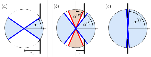
Figure 2. Geometrical connection between the centre-of-mass position x and allowable rotation angles, for three characteristic examples of a classical rotor passing through or reflected from a slit. Here we have chosen the ratio of rotor length to aperture size to be  .
.  Rotor geometry when the rotor tip just touches the openings of the slit. This position,
  , with
  , marks a critical moment in the motion of the rotor towards the slit. Here the rotation angle φ first becomes hindered, constrained to the domain
  .
.  For smaller separations
  there are two domains of allowed angles. For rotors that are on their way through the slit the rotation angle
  is constrained by the angle
  This region is shaded blue. For rotors to be reflected the angle
  must lie within a domain located symmetrically around
  and of width
  where
where  This region is shaded red. The frame depicts
  .
.  Rotor geometry when the rotor is centred in the slit, at x = 0. Here the domain of reflection angles vanishes, i.e.
  . The rotor is essentially free, i.e.
  , provided the slit is infinitely thin. However, the rotor cannot complete a full rotation.
Download figure:
Standard image High-resolution imageIn (3) we have introduced the aperture-to-length ratio

This parameter plays an important role throughout this article.
2.2. Classical constraints
A classical rotor can only pass through the slit (be transmitted) if its angle  at
at  obeys the inequality
  where the critical angle is

For all other angles the classical rotor will be reflected.
While the rotor is passing through the aperture its rotation is hindered. An elementary geometrical argument shows that for a rotor at position  the angle
  is, in transmission, restricted by the inequality

where

Likewise, a rotor at position x will be reflected if its angle  fulfills the inequality

where

As is evident from figure 3, rotation angles between  and
and  cannot occur.
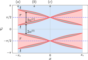
Figure 3. Geometrically allowed domains (red and blue) and forbidden domains (dark grey) of rotation angles φ corresponding to reflection (r) and transmission (t), respectively, for a rotor with  . The figure shows angles
  associated with positions x of the centre-of-mass of the rotor within the region
  where the rotation becomes hindered by the slit. Rotors approaching from
  will be transmitted or reflected depending on whether
  lies within region t (blue) or r (red) , respectively. At a given position x the widths of the allowed angular intervals corresponding to the transmitted and reflected particles are, respectively,
  of (7) and
  of (9). The three locations
  ,
,  and
and  of the rotor from figure 2 are indicated on the frame top .
Download figure:
Standard image High-resolution image2.3. The classical transmission probability
We conclude our discussion of classical motions by noting that in the stream of particles in the rotational ground-state that impinge on the screen only those rotors pass through the aperture whose angle of orientation φ lies within the interval  . All other rotors are reflected. Hence the classical transmission probability
  i.e. the ratio of the number of transmitted rotors to the number of incident rotors, is determined by the ratio

For a symmetric rotor, as we consider, the physical structure is unchanged if the particle is rotated by π. Hence the denominator of the ratio in (10) is π. From (5) we find the numerator, i.e. the domain of rotor orientations that allows classical transmission, to be  . The resulting formula reads

In the limit of a rotor size a approaching the aperture size b, that is for  , we find
  and hence
  , i.e. all rotors are transmitted, as expected.
In the remainder of the paper we concentrate on the modifications of the classical transmission probability introduced by quantum mechanics. We show that the classical transmission can be enhanced or suppressed. We also find that the rotor can be (temporarily) trapped within the aperture. This delay of progress through the aperture is visible as enhanced wavefunction density within the aperture and as a resonance increase in transmission; the width of the resonance is inversely proportional to the delay.
3. Quantum particles with internal structure
The foregoing discussion of the scattering of a classical rotor from a slit in a thin screen only involved geometric relationships between the length a of the rotor and the size b of the aperture, as expressed by the aperture-to-length ratio  . The mass-distribution parameter
  of (1) plays no role in such geometrical constraints. The reason for that is the following. We are concerned with rotors whose initial motion, far from the screen, is entirely translational. Then the initial classical angular momentum
  vanishes, and the rotational contribution to the Hamiltonian vanishes as well. Consequently the factor
  , which contains the
  -dependence, has no effect classically and only the lengths a and b are needed to completely characterize the scattering.
By contrast, quantum mechanics allows the parameter  to affect the scattering process even for rotors that are initially not rotating. Although the length a quantifies the extent of the structured particle as it interacts with the slit, a second parameter is needed to express the distribution of mass. For example, in a diatomic molecule the mass is concentrated in two nuclei, whereas the size of the molecule is determined by the distribution of electron charge. The nuclei are essentially point charges, whereas the electrons are essentially massless. The mass-distribution parameter
  is the ratio of the length of the electron distribution to the internuclear separation. It has maximum value,
  , when the mass is concentrated at the two ends.
In the quantum-mechanical description the classical Hamiltonian becomes a differential operator. The rotational kinetic energy operator is proportional to the second derivative of the wavefunction with respect to the angle φ and, as we shall explain below, this introduces an explicit dependence upon the mass-distribution parameter  .
.
In the present section we show how the classical constraints discussed in the preceding section translate into boundary conditions on the energy wavefunction describing the centre-of-mass motion and the rotation. We then eliminate the rotational degree of freedom in the interaction region and derive a series of effective potentials for the motion along the x-axis.
3.1. The quantum rotor
Our quantum mechanical model is that of a symmetric rigid rotor. That is, we allow rotation of the molecular framework but neglect the possibility of vibrational motion that would alter its dimension. This is a reasonable approximation as long as the initial translational energy is much lower than the energy of the lowest-lying vibrational excited state. Vibrational excitation energies are significantly larger than rotational excitation energies, and so our analysis is consistent with the assumption of a rigid rotor. As we will note in a concluding section, our outlook offers some possible physical examples of molecules that might be suitable candidates for the scenario we discuss.
We assume that the incident particles are in their rotational ground state. As with the classical rotor, we consider a quantum rotor whose axis of rotation (i.e. the quantization axis) is perpendicular to the velocity, which we take to be in the x direction. We consider an apertured screen that is perpendicular to the velocity, at x = 0, and we simplify the centre-of-mass motion to be along a track through the centre of the aperture. Thus the translational motion requires only one degree of freedom (coordinate x) , as does the rotational motion (coordinate φ).
3.1.1. The quantum Hamiltonian
The energy wavefunction  for the moving rotor is determined, for translational and rotational variables x and φ respectively, by the time-independent Schrödinger equation,

The quantum mechanical Hamiltonian operator  appearing here follows from (2) by replacing the classical momenta px and
  by differential operators, respectively
  and
and  . As a result, the time-independent Schrödinger equation (12) describing the scattering of a fixed-energy rotor from a slit becomes the partial differential equation

This is the two-dimensional Helmholtz equation for variables x and  . It must be supplemented by appropriate boundary conditions. As we next explain, these incorporate the quantum counterpart of the geometric restrictions of classical rotation.
3.1.2. Dimensionless scaled variables
To identify the relevant parameters and get a dimensionless eigenvalue equation it is convenient to express the energy E of the incoming rotor in terms of the energy  of the rotor discussed in appendix

We introduce a dimensionless measure of distance s by expressing the position variable x in units of the effective rotor length  ,
,

With these definitions the Schrödinger equation reads

where we see on the left the two-dimensional Laplace operator in the variables s and φ.
When distances are expressed in terms of the dimensionless variable  then the critical distance
  where the rotor begins to be affected by the screen,

is adjusted by the aperture-to-length ratio  and is inversely proportional to the mass-distribution parameter
  . With these modifications the geometrical constraint of (6) for the transmission domain becomes

where

while (8) for the reflection domain reads

where

These considerations show that the relevant parameters describing the geometrical situation are  and
and  .
.
3.1.3. The incoming free rotor
The rotor Hamiltonian of (2) is the sum of two kinetic energies: translational and rotational. When the rotor is far away from the screen the translational and rotational degrees of freedom are uncoupled. The energy wavefunction  is then expressible as a product of a plane wave, corresponding to the centre-of-mass motion, and an eigenfunction of a free rotor—one that can experience unhindered rotation.
We confine our analysis to rotors that are initially in the rotational ground state, of zero rotational energy, as specified by vanishing angular momentum quantum number m discussed in appendix  arises entirely from the initial translational kinetic energy and the wavefunction is separable: we write it as the product of translational and rotational wavefunctions

where  . The rotational label
  indicates that the rotation is unconstrained. Upon entering the aperture the rotation becomes constrained and such a product must be replaced by a wavefunction that incorporates such hindrance
  , see appendix
3.2. Coupled mode-functions
When the rotor enters the interaction region , where  , its rotation becomes hindered. Although the rotor remains in the rotational ground state, the rotational eigenvalue increases as the motion becomes more restricted. We treat this hindrance by requiring that the rotational wavefunction vanishes for angles that lie outside the domain of classically allowed motion, given by (19) and (21). Figure 3 displays an example of the allowed domains of φ. The hindered motion, and the resulting entanglement of variables
  and φ, we incorporate by imposing the boundary condition that the wavefunction should vanish at the borders of the allowed angular domain.
We now derive a system of coupled equations for the wavefunctions of the centre-of-mass motion. The coupling arises from the position dependence of the boundaries. We then specialize these equations to treat transmission.
3.2.1. Quantum constraints as boundary conditions
Figure 3 shows that the allowed angular motion of the particle separates into two domains, transmission  and reflection
  . It is necessary to consider separately the wavefunction for these two domains. In either one the angle φ lies between two position-dependent values

The boundaries of the allowed range of angles,  and
and  and the width
  differ for transmission and reflection domains. For the transmission domain we find from (18)

For the reflection domain we identify

As shown in appendix

and  and
and  are given by either (24) or (25). Here we have omitted the superscript
  indicator of hindered motion used in appendix
3.2.2. General mode equations
Using the hindered-rotor wavefunctions (26) we make the ansatz

We substitute this into the Schrödinger equation (16). After working out the derivatives we project the resulting equation onto each hindered-rotor wavefunction  . We arrive in this way at the system of differential equations for the translation functions
  ,
,

where primes denote differentiation with respect to the translation variable s. Expressions for the arrays Amn and Bmn are given in appendix  and
and  .
.
Three features stand out in (28). First, the bracketed term multiplying the Kronecker delta  represents a semi-independent Schrödinger equation for the centre-of-mass motion with the fixed initial energy
  in an effective potential

determined by the dependence of the boundary angle  on position s.
Second, the position dependence of the boundary, through  , gives a position dependence to the hindered-rotor wavefunction
  and thereby leads to a coupling of the modes, expressed in the second line of (28) by terms proportional to the constant arrays Amn and Bmn.
Third, the spatial dependence of these couplings appears in the ratios  and
and  , which vanish for boundaries that do not depend on s. The remaining portions of the couplings, the matrices
  and
and  , are independent of position.
3.3. Mode-decoupling approximation
To obtain useful analytical results we neglect the sharp changes in  at
at  and s = 0 thereby neglecting the ratios
  and
and  . This assumption allows us to neglect the mode coupling in (28) and deal with a set of independent equations for the centre-of-mass motion. In this approximation each translational mode function
  becomes effectively decoupled from all the others, obeying the equation

Here we use (21) to express the effective potential for the reflection as

while we use (19) to write the effective potential for the transmission as

The expansion (27) of the total wavefunction in the two variables is fundamentally, and crucially, different in the regions of free and hindered rotation. Therefore we cannot consider these potentials as part of a total potential extending from  to
to  in
in  . They serve only to determine the wavefunction inside the
  region, while the usual fitting of the solutions (i.e. matching functions and derivatives) is to be performed for the total two-dimensional wavefunctions. The full domain of centre-of-mass positions we divide into three regions: in region I the particle approaches the slit, unhindered by any walls. In region
  the particle continues moving beyond the slit, again unhindered. In the intermediate region,
  , the wall hinders rotation and there is a correlation between translational and rotational degrees of freedom.
3.4. Properties of the effective potentials
Next we discuss the forms of the two effective potentials  and
and  scaling with n2 for higher modes (30). We first analyse their general features and then illustrate them in figure 4 for certain values of c and a fixed
  . In particular, we examine limiting cases of the potential.

Figure 4. Effective potentials  (top frame), from (31), and
  (bottom frame), from (32), versus scaled centre-of-mass coordinate
  for
for  . Dashed blue lines are for
  while red lines correspond to c = 0.9. The potential
  responsible for reflection displays an infinite barrier at
  , whereas the potential
  responsible for the transmission displays a minimum at this point. Note that these potentials make sense only in the region
  (
( ), as indicated by dotted vertical lines. We emphasize that the domain of
  depends on c.
Download figure:
Standard image High-resolution image3.4.1. Reflection potential
It is important to note that the reflection potential  given by (31) does not depend explicitly on the aperture-to-length ratio
  . This parameter affects the potential only implicitly: it changes the position
  of the boundary which, according to (17), depends on c as well as on
  . The consequence of this property is evident in the top frame of figure 4, where we show
  for c = 0.5 and c = 0.9. At the end points of the region,
  , the height of the reflection potential,

is independent of the mass-distribution parameter  . When the aperture is much smaller than the particle size this value approaches unity,

In the opposite limit, when the aperture is only slightly larger than the rotor we find

This value becomes large without limit as c tends towards 1 and the rotor fills the slit. However, in this limit the domain boundary  also tends to zero, because
  . This behaviour expresses the fact that near the centre of the aperture, at
  , the reflecting potential becomes unboundedly large,

3.4.2. Transmission potential
We now turn to the transmission potential  , given by (32). In contrast to the reflection potential
  the transmission potential depends explicitly on the parameter c. However, as in the case of the reflection potential (33), the limiting value of
  at
at  , of height

is again independent of  . In the limit of a small aperture this expression tends to

As the particle approaches the centre of the slit  decreases. In the neighbourhood of the centre of the aperture we find from (32), with the help of the asymptotic expansion
  , valid for
  , a linear dependence of the potential on distance away from the centre

The value of  at the aperture centre,
  ,
,

corresponds to the scaled energy  of a hindered rotor that has complete access to all angles. The steepness of the linear potential in (39) is proportional to
  as well as to
  . Notably, the potential
  at
at  is non-differentiable. Indeed, the
  -variation of
  exhibits a kink (or corner) [4, 20] at the centre of the aperture.
For distances further away from the centre of the aperture, we use a linear approximation to the  function, thereby obtaining from (32) a quadratic expression for the transmission potential,

That is, the transmission potential is that of a harmonic oscillator. We note that when  the boundary becomes
  and so for
  expression (41) correctly yields the limiting potential value
  predicted by (38). Hence we can fit a quadratic function

to the potential  . As can be seen from figure 5 there is deviation from this quadratic form only around
  where there is a kink. This harmonic oscillator approximation will play an important role in section 4 where we discuss the quantum-mechanical transmission.

Figure 5. The effective potentials  and
and  versus scaled centre-of-mass distance s. Dashed red line is
  . Fitted quadratic oscillator potential
  is a continuous blue line. Parameters are c = 0.5 and
  .
.
Download figure:
Standard image High-resolution image3.5. The scattering equations
For further simplification we modify the boundary conditions by requiring that the wavefunction vanish at  for
for  and for
  , as shown in figure 6 by the vertical red lines. This modification has no influence on the quantum-mechanical transmission probability because particles can only pass through when φ is within the interval
  marked by the vertical dotted lines. For this reason we will focus on
  , which is nonzero only in the unshaded region
  in figure 6.
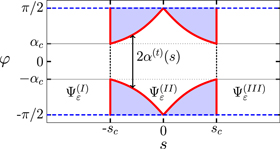
Figure 6. In regions  and
and  the rotation is uninhibited, while in region
  it is hindered. The boundary of region
  is given by
  defined in (19). The free rotor solutions describing an incoming wave from the left, with the transmitted and reflected part as well, is given by
  defined in (43) and
  defined in (48). In the interaction region, where the rotation angle is restricted, the wavefunction
  is given by (47). The two boundaries where the fitting should be done are at
  defined in (17). The red line marks the modified boundary where the wavefunction must vanish, while the dashed blue line reminds us of the periodic boundary condition.
Download figure:
Standard image High-resolution imageIn the region I the wavefunction is a superposition of a single right-going initial wave of unit amplitude and several reflected waves of relative amplitudes  , a property we express by the ansatz

Note that in (43) the indices  corresponding to the different rotational wavefunctions of the free rotor,

run from  to
to  . In specifying the system we consider a fixed initial scaled energy
  of the rotor approaching the aperture. Because the scaled energy is the sum of the translational energy km2 and rotational energy
  (see (A.22)),

it follows that for  the higher modes are exponentially decaying functions, with kinetic energy parametrized by

It is essential to include these non-oscillating functions when we fit the incoming plane wave (22) with sinefunctions extending from  to
to  at the left and right boundary of region
  .
.
Continuing the ansatz (27) we replace  by a linear combination of two independent solutions
  and
and  of (30) and write the wavefunction in region
  as
as

with constant coefficients an and bn. The effective potentials in (30) are even functions of s so we can choose one of the solutions (fn) to be even while the other (gn) is odd. However, we retain the wavefunctions  of the hindered rotor, defined in (A.13). Note that in (30) and hence in (47) the parameter
  is set a priori by the energy of the incoming wave (22).
In principle we can get the fn and gn solutions numerically with the original effective potential (32). But as we have seen in section 3.4 the potential  can be approximated by the quadratic form of a harmonic oscillator potential. The equations for these approximate oscillator potentials (41) can be solved analytically by infinite sums (see [27] for example).
Finally, in the region  there are only transmitted waves, with relative amplitudes
  , and we use the ansatz

At the boundary  we require continuity of the wavefunctions and continuity of the derivatives, see Appendix
  .
.
From rm and tm the transmission and reflection coefficients for the probabilities of transmission T and reflection R are obtained as

Note that we have allowed exponentially decaying functions so km is not necessarily real.
4. Results: tunnelling, trapping and resonances
In this section we present results obtained from the solutions of the Schrödinger equation (16) based on the approximations introduced in section 3.3. Specifically, we use here the approximate oscillator potential (41) to solve the one-dimensional equations of (30) analytically. In spite of the numerous approximations in our present treatment, the results obtained are surprisingly accurate, as we have confirmed by obtaining numerically exact solutions of the Schrödinger equation on a discrete lattice with the boundary conditions shown in figure 6 [13]. Those calculations, shown as dashed lines in the figures below, constructed the Green's function of the system on a suitably chosen finite-sized discrete lattice. From the Green's function we evaluated the S-matrix of the problem and in turn the transmission and reflection probabilities as a function of energy.
4.1. Energies below the potential minimum: tunnelling
Quantum-mechanical waves, like electromagnetic waves, exhibit two characteristics that are alien to classical particles: interference and tunnelling. Both phenomena are observable in the present scattering problem. At very low energies,  , it is not possible to have positive kinetic energy, meaning
  , anywhere within the interaction region
  , and so a classical particle cannot be found there. A quantum particle can, however, tunnel through such a classically forbidden region. At energies
  the potential provides a barrier of width
  independent of further decrease of energy. Therefore one expects a tunnelling probability that decreases exponentially with decreasing energy. Figure 7 shows, for
  and two values of c, that indeed this is the behaviour of the transmission for extremely low energies,
  .
.
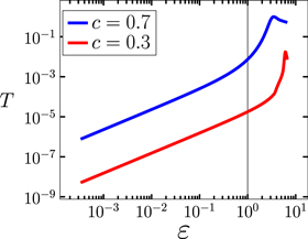
Figure 7. Transmission probability T versus scaled centre-of-mass energy  plotted in logarithmic scale, showing exponential variation associated with tunnelling through the barrier provided by
  . The energy range here goes extremely far below the minimum of the potential,
  . Parameters are
  , c = 0.7 (upper curve) and c = 0.3 (lower curve).
Download figure:
Standard image High-resolution image4.2. Energies below the barrier height: trapping and resonances
At energies above the potential minimum,  , classical motion can occur within at least a portion of the interaction region. However, the classical rotor will be reflected by barriers at
  . The presence of two potential barriers in a one-dimensional scattering equation allows solutions analogous to a Fabry–Perot interferometer in which the wavefunction is almost entirely confined between the barriers. The transmission potential
  can, for suitable parameter choices, provide such confinement. For the elementary example of a free particle encountering two very thin barriers the requirement for this wavefunction localization is that an integer number of half waves should fit within the walls.
To quantify the energies which produce rotor localization we recall from (42) the fitted harmonic oscillator potential  that agrees very well with
  away from
  ,
,

Here we have made use of (40) and have introduced the oscillator frequency

This model oscillator has the quantum-mechanically allowed energies

where the number of oscillator states nmax is the integer obtained as the lower bound

The potential  is nonzero, i.e. confining, only within the region
  , and hence it is only within this region that the quadratic approximation can hold. This means that energies
  above
above  lie above the barrier. Energies greater than this value would allow classical particles to pass freely over the barriers. We can expect that oscillator energies below this value will provide an approximation to the scattering energies for which the wavefunction exhibits strong localization (bound states) manifested by resonances in the transmission probability. The number nmax is an excellent approximation to the number of these discrete bound states in the transmission potential.
Figure 8 displays the low-energy regime  for the parameter choice c = 0.4 and
  . Frame
  shows the transmission potential
  (dashed grey). The peak of this potential barrier corresponds to an energy vc = 14.57. The solid (blue) curve is the fit
  of a quadratic potential to
  . It is only appropriate within region
  , where
  . The thick-black and thin-black horizontal lines mark the harmonic-oscillator energies for this potential: there are two of them below the barrier of height vc. Frame
  shows the transmission probability T as a function of scaled energy
  as obtained from the oscillator approximation (solid curve) and from exact numerical calculations of [13] (dashed curve). The validity of the oscillator approximation is evident in the good agreement between the two plots in frame
  . Indeed, the resonance peaks are very close to the energy eigenvalues of the fictitious oscillator. The lowest-energy peak, corresponding to the lowest-energy bound state in the potential well, is notably narrower that the peak at higher energy, which occurs at the top of the potential well. The exact calculations [13] shift the resonance energy upward from the prediction of the oscillator model. We suspect this shift is a consequence of the kink in the exact potential. According to [4] such corners create secondary waves which superpose with the original wave to produce a phase shift in the total wavefunction. In turn this causes an energy shift.
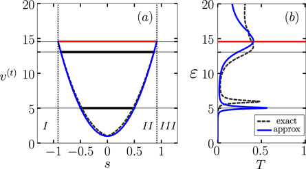
Figure 8.
 Potentials
  (dashed grey line) and vosc (solid blue line) versus scaled centre-of-mass coordinate
  . Horizontal black lines (thicker inside the well) mark the energies of the first two harmonic oscillator states. The horizontal red line marks the barrier height
  .
.  Transmission probability T versus dimensionless energy parameter
  . The thick curve is obtained from the oscillator approximation, the dashed curve is from a numerically exact calculation [13]. The first two peaks approximately correspond to the the oscillator energies. Parameters are
  , c = 0.4.
Download figure:
Standard image High-resolution imageOur studies of wavefunctions [13] have confirmed that at the energies where there appears a resonance in the transmission the wavefunction is much larger inside the region  : the particle is 'trapped' within the aperture. The sharper the resonance the more strongly localized is the wavefunction.
4.3. Energies above the barrier: effect of rotor size
As the aperture-to-length ratio  increases the heights of the two barriers decreases and fewer harmonic-oscillator states lie below the barrier height vc. Consequently the resonances become broader and less distinct. Figure 9 shows examples of transmission probability for parameters that allow only a single bound state, over an energy range that extends well above the barrier and four choices of the aperture-to-length ratio c.
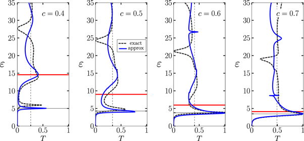
Figure 9. Transmission probability T as function of scaled energy  for
for  and four values
  of the aperture-to-length ratio
  . Dark blue curves show the results from the oscillator approximation, while dashed grey curves are the results of the exact numerical treatment [13]. Thin horizontal lines mark the ground-state energies of the approximate oscillators. The horizontal red lines indicate the top of the potential barrier above which there are no bound states (cf. figure 8). Dashed, grey vertical lines provide the classical transmission probability
  of (11).
Download figure:
Standard image High-resolution imageAs can be seen in figure 9, the harmonic-oscillator eigenenergies, marked here by thin horizontal lines, fit the energies of resonances in the transmission probability. The oscillator model correctly predicts that as c becomes smaller and the potential becomes larger at the edges, the resonance becomes sharper. Exact numerical calculations [13], shown as dashed grey curves, predict that as the aperture-to-length ratio c diminishes, with consequent broadening and steepening of the potential, the resonance energy shifts slightly upwards.
For energies above vc, denoted by the horizontal red line, where classical particles would move freely, there is little structure in the solid curves predicted by the oscillator model. However, the exact calculations (dashed lines) reveal a distinct dip in transmission probability. This shifts towards higher energies as the aperture-to-length ratio c becomes smaller. Our computation of wavefunctions [13] show that such minima are not examples of the broad Ramsauer–Townsend minima seen in electron scattering [46] nor the Cooper minima observed in photoionization [10, 45].
4.4. Energies above the barrier: effect of mass distribution
The dynamics of the quantum-mechanical scattering brings in a second independent parameter,  , expressing the distribution of mass (as it influences the rotational kinetic energy) relative to the size of the particle as probed by the interaction with the slit. According to (37) the height of the transmission-potential barrier vc does not depend on
  . However, the width does: with fixed rotor and aperture size (fixed c), a decrease of
  broadens the potential. This means that more oscillator eigenenergies fit into the energy domain
  . In turn the resonance peaks associated with these eigenenergies are more closely spaced and narrower with decreasing
  .
.
Figure 10 shows examples of the energy dependence of the transmission probability, for four values of the mass-distribution parameter  . Quite notable in the left-hand frames are resonances for energies above the top of the oscillator well, indicated by the horizontal red line. The exact calculations do not show such sharp resonances. Instead we see continuum structure marked by transmission dips. These become sharper as
  decreases. We attribute this difference to our neglect of the derivatives
  and
and  in (28), made in obtaining the decoupled-mode equation (3.3) and the effective potentials used there.

Figure 10. Transmission probability T as a function of scaled energy  for fixed aperture-to-length ratio
  and values
  of the mass-distribution parameter. The horizontal red lines mark the top of the barrier above which there are no bound states, see (37). A decrease of
  , with c fixed, broadens the width of the potential barrier. This change decreases the energies of the resonances. As the potential becomes wider, the area under the tunnelling barrier increases and consequently the transmission lessens. Dashed, grey vertical lines provide the classical transmission probability
  of (11), independent of
  .
.
Download figure:
Standard image High-resolution image4.5. Predictive power and accuracy of the oscillator model
From figures 9 and 10 we see that our oscillator approximation, while it gives very well the energies where resonance peaks appear, loses the information about the value of T at the resonances. This disagreement originates from our neglect of coupling between modes.
A comparison with the numerically exact solutions [13] shows that the effective oscillator potential provides a good approximation for the low energy behaviour and this potential quantifies well the low-energy resonances. The weakness of this approximation is apparent in results for transmission at higher energies, as seen in figures 9 and 10: the effective oscillator cannot explain the transmission dips that exact numerical solutions show, and it predicts sharp resonances that are not seen with the exact solutions.
5. Outlook and conclusions
In this section we summarize our results and discuss the requirements on the energy of the centre-of-mass motion of the rotor. We analyse the limitations of our elementary model, briefly suggest possible extensions and list possible candidates for experiments that might reveal some of the phenomena reported here.
5.1. Summary
The present article discusses the scattering of a particle with some internal structure, specifically a rigid rotor, from a single slit in a thin but impenetrable barrier. We have focused on the situation in which the length of the rotor is larger than the size of the slit. In this case the hindered rotation imposes non-trivial constraints on the centre-of-mass motion and leads to a complicated system of differential equations. A smoothing approximation of the constraint conditions simplifies the model to a set of uncoupled equations (30), which reformulate the constraints as effective potentials, for transmission and for reflection.
The reflection potential is a simple barrier, but its extreme height at the aperture centre prevents any tunnelling. The transmission potential has a maximum when the rotor first interacts with the screen, has a minimum when the rotor is in the centre of the aperture, and increases again as the rotor moves further through the aperture. The double-barrier form of the potential allows resonances in the transmission probability as a function of incident kinetic energy. At these resonance energies the wavefunction becomes enlarged within the aperture-interaction region, that is, the rotor becomes trapped within the aperture. The trapping arises from the wave nature of the rotor and from the coupling between the translational and rotational degrees of freedom induced by the screen. Our smoothing approximation is a simplification which describes well the physics of a non-rotating incoming object in the low energy regime. It also allows us to calculate the energies where resonances occur i.e. where a significant enhancement in transmission appears.
For incident energies below the effective barrier one can gain a satisfactory description of trapping resonances by approximating the effective potential as a quadratic function of the centre-of-mass position, and treating the harmonic-oscillator states of that potential as approximations to the actual wavefunctions. There can only be a finite number of bound states, each of which produces a resonance in the transmission probability.
The scattering wavefunctions used in these calculations are constructed as sums of analytic basis functions. We emphasize that these sums include not only sinefunctions, which vanish on the boundaries, but also include evanescent (exponentially decaying) waves.
5.2. Energy requirements
We now address the relationship between the scaled variables used to simplify the physics and the lengths and energies that will occur in any practical application of the theory.
According to our analysis the most evident quantum mechanical modification of the classical transmission probability  given by (11) occurs when the scaled energy
  is smaller than, or of the order of, the maximum value
  of the transmission potential at the critical separation
  , i.e. for
  . In the limit of a small aperture-to-length ratio
  we find from (36) and the definition (14) of
  , that the scaled energies must be small,

It is useful to convert this condition into unscaled energies.
As shown in appendix  . Consequently, we find that the classical scattering of the rotor begins to be influenced by quantum effects for initial energies

Because we consider the aperture size  to be smaller than the rotor size
  , the pre-factor can be larger than unity. For example, for
  the pre-factor is
  . Hence the modification of classical scattering sets in for energies E which are up to twice the energy of the first rotationally excited state.
The wave nature of the translational motion is characterized by the de Broglie wavelength

where we have recalled in the last step the definition (14) of the scaled energy . The low-energy resonances occur for large  . The energy condition of (54), when expressed in terms of
  , reads

thereby exhibits a relationship between centre-of-mass speed and the basic parameters of the model, namely:  the size a of the rotor;
  the rotor mass distribution, expressed by
  ; and
; and  the aperture-to-length ratio c. Pronounced resonance effects occur primarily for
  and
and  , and so the condition for resonances is that the de Broglie wavelength be larger than the rotor radius a times a factor that is less than unity.
5.3. Caveats
Any application of our elementary model of a quantum-mechanical travelling-rotor must take note of several limitations. A basic shortcoming of the present elementary model is the restriction to a single translational degree of freedom: the centre-of-mass follows a track through the centre of the aperture. In reality, projectile motion is three-dimensional. Quantum mechanics in two and three dimensions is certainly very different from that of one dimension, and many modifications of our model will arise with the inclusion of additional dimensions. These complications fall beyond our present mandate.
Our model, embodied in the Schrödinger equation (30), assumes that the different translational modes are not coupled to each other by the constraints. An alternative approach avoiding this complication based on the Green's function of the problem is to be presented in a forthcoming publication [13].
5.4. Experimental prospects
Recent years have brought enormous progress in experimental techniques that enable the scattering of particles with internal structure from gratings whose spacings are comparable to the size of the projectiles. Helium clusters are candidates for projectiles. Helium dimers, for example, can be as large as 5 nm [28]. Moreover, they occur only in rotational ground states. The Efimov state of the helium trimer, if it exists, is expected to have a size of 8 nm [37].
Mechanical gratings are available with spacings of 100 nm or less. By tilting a grating the effective aperture can be reduced considerably. As shown theoretically and experimentally the resulting slit width of a grating whose spacing is 100 nm can be reduced to a few nm [8, 30]. When we recall that the Efimov state in helium is of the order of 8 nm, the desired inequality, (57), is within reach. However, the de Broglie wavelength of helium experiments at room temperature (less than 0.1 nm) are too small [30] so lower temperatures are needed. Moreover, the atom-surface van der Waals potential from the grating could mask the effects of interest [29].
Another possibility for small apertures could be nanoscale sieves. These have been used to measure the transmission of helium dimers [44].
Optically trapped dimers, such as Li2 or Cs2, formed by three-body recombination of ultracold atoms by a magnetic field-induced Feshbach resonance offer another approach towards realizing suitable projectiles. These weakly bound structures have a remarkable size which depends upon the strength of the magnetic field [36]. Even the Efimov states of cesium might be possible candidate projectiles [39].
Size-selected short carbon nanotubes might be used as structured projectiles. However, here a serious challenge would be to create a well-defined rotational state.
Another experiment, performed on molecules of perfluoroalkyl-functionalized azobenzene [22], has demonstrated the wave nature of the centre-of-mass motion of an elongated molecule. These molecules appear in cis and trans configurations, and the transition between these two configurations can be induced by uv radiation. In the trans form this molecule has a length of 3 nm but is only a few tenths of a nm wide. Such a molecule could be a possible realization of the straw of the Ulm sparrow [34]. In this experiment [22] the molecules were in highly excited rovibrational states. The research group has also conducted an experiment [34] using a classical Talbot-Lau interferometer for a beam in which only a few rovibrational states are populated. Moreover they plan [34] to switch between cis- and trans-configurations, thereby altering the rotor length. In this way they can observe the influence of the mass distribution.
The idealization to an infinitesimally thin aperture whose chemical properties have no effect might be created by suitable laser fields. Indeed, in the study of atom optics [1, 2] gratings based on appropriately tailored laser beams are a standard technique.
We conclude this discussion of the experimental prospects by alluding to a recent experiment [12] demonstrating a novel method for probing the alignment of the molecular axis of an ultracold, nonpolar dimer. Indeed, [12] reports the preparation of Rb2 molecules trapped in a three-dimensional optical lattice in various precisely defined rotational quantum states. Although in these experiments the molecules were in the vibrational ground state with an internuclear separation of about 6.09 Angström, to engineer the alignement of the rotational axis of an ensemble of ultracold molecules represents a major step towards the realization of the Ulm sparrow.
5.5. Conclusion
Our article has examined a simple model of classical and quantum scattering of a particle that has internal structure, specifically that of a rigid rotor, from a single slit in a thin wall. The transmission of the quantum particle through the slit exhibits resonances that can be understood qualitatively by means of a harmonic-oscillator approximation. A key result is that boundary conditions at the slit lead to entanglement of rotational and translational degrees of freedom.
Experimental progress in creating cold molecular beams makes us confident that our toy model representing the quantum version of the Ulm sparrow can be realized in an experiment.
Acknowledgments
We acknowledge enlightening, stimulating and useful discussions with M Arndt, MG Benedict, L Cederbaum, O Crasser, P Exner, P Földi, P Fulde, R J Glauber, R Grimm, P Julienne, A A Krokhin, N Moiseyev, R F O'Connell, V L Pokrovskii, H Rauch, G Shlyapnikov, E Tiemann, J P Toennies, J Tolar and P E Toschek on various aspects of this work. We gratefully acknowledge funding from the Baden-Württemberg Stiftung through the Atomics Program, from the SFB/TR21 'Control of quantum correlations in tailored matter: common perspectives of mesoscopic systems and quantum gases' and from the EU through the research and training network EMALI (MRTN-CT-2006-035369). The work of PD was supported by the European Union and the European Social Fund through projects 'Supercomputer, the national virtual laboratory' (Grant No. TAMOP-4.2.2.C-11/1/KONV-2012-0010) and 'Impulse lasers for use in materials science and biophotonics' (Grant No. TAMOP-4.2.2.A-11/1/KONV-2012-0060), and by the Hungarian Scientific Research Fund (OTKA) under Contract No. T81364. WPS thanks the Alexander von Humboldt Stiftung and the Max Planck-Gesellschaft for receiving the Max Planck-Forschungspreis. Moreover, he is grateful to Texas A&M University for a Texas A&M University Institute for Advanced Study (TIAS) Faculty Fellowship. BWS acknowledges support from funds available through the Max Planck-Forschungspreis 2003 awarded to Klaas Bergmann and from the Deutsche Forschungsgemeinschaft in Kaiserslautern. Portions of this work were presented by WPS at a 70th Birthday Symposium for BWS in Kaiserslautern, 2005.
Appendix A.: Wavefunctions of rotation and translation
In our analysis of the scattering of a symmetric rigid rotor from a narrow slit we build the wavefunction from products of functions that describe the rotation and others that describe the centre-of-mass motion. This appendix describes these wavefunctions and builds the two-dimensional wavefunction  and
and  from them.
A.1. The rotation equation
The rotational wavefunctions are solutions to the equation

Here  denotes the dimensionless rotational-energy eigenvalue in units of

To complete the equations we must supply boundary conditions on the φ dependence. In so doing we distinguish two classes: those in regions I and  where the the rotor is free to rotate fully, leading to wavefunctions we denote as
  , and those in region
  where the rotation is hindered, i.e. restricted to a finite range of angles, denoted as
  . Those hindered-rotor wavefunctions we further classify as referring to the domain of transmission,
  , and rotation,
  . As will next be shown, for each of these the solutions form a discrete set of rotational mode functions.
A.1.1. The free rotor
A satisfactory wavefunction for a free rotor, i.e. a solution to (A.1) in regions I and  , can be written

where  is a normalization constant. From (A.1) it follows that the rotational eigenvalue
  for the free rotor is

The physical configuration of a symmetric rotor, as considered here, is unchanged if it is rotated by π about its axis (for asymmetric rotors the needed angle is  ). It follows that the wavefunctions for an unhindered symmetric rotor must be odd or even under such a rotation. In our analysis we confine our attention to the even class, which contains the ground state.
We therefore consider functions that satisfy the periodic boundary conditions

This condition, taken with the functional form of (A.3), leads to the condition that the allowed values of  form a discrete set of values
  such that

where m is a positive or negative integer or zero. As a consequence, the allowed rotational energies of a free rotor are

The corresponding free-rotor wavefunctions, normalized on the interval  , are
, are

The functions for which m is a positive integer represent counterclockwise motions; for negative m they represent clockwise motions.
According to (A.7) the lowest-energy state of free rotation, associated with m = 0, has vanishing rotational energy,  . The corresponding wavefunction
  defined by (A.8) is a constant; in this state all angles φ are equally probable.
A.1.2. The hindered rotor
Within region  the orientation of the rotor is constrained to lie within a finite range of angles,

and so the hindered-rotor wavefunctions must vanish at the borders  and
and  . With the imposition of these boundary conditions the wavefunctions and the energy eigenvalues acquire implicit spatial dependence through the dependence on
  . Then (A.1) becomes

Here  is the dimensionless energy eigenvalue, dependent on s through the boundary condition.
For a given position s and domain  a satisfactory trial expression is

This construction automatically obeys the boundary condition at  and can be made to satisfy the condition at
  by requiring that the allowed values of
  form a discrete set, fixed by the condition

where n is an integer. The null function obtained with n = 0 is not an admissible wavefunction. Hence we obtain the expression

where we have determined the normalization constant  for the allowed position-dependent angular interval
  . A change in sign of n produces only a change in sign of
  . Therefore we restrict the wavefunctions to positive values of n.
The functions (A.13) satisfy the orthonormality relations

These functions obey the Schrödinger equation (A.1) subject to the requirement that the rotational energies form the discrete set

These are the allowed rotational energies of a symmetric rigid-rotor whose angular orientation is restricted to the range (A.9). Significantly, according to (A.15) the non-vanishing wavefunction with lowest energy is that with n = 1.
A.1.3. Comparison
The two classes of rotors discussed above, free and hindered, each have eigenenergies  proportional to
  . However, the energies differ in three features:
- (1)in the factors multiplying m2 or n2, i.e. 4 versus
 ;
; - (2)in the restriction to positive n-values for the hindered rotor; and
- (3)in the possibility of m = 0 for the free rotor, a choice that is not allowable for the hindered rotor.

Moreover, the two classes of rotational wavefunctions, though both discrete, differ significantly, as required by the different boundary conditions.
In the limit of  the range of the hindered rotor becomes
  , and the factor
  of the hindered rotor becomes unity. Although the range of angles is then equal to that of the free rotor, the different boundary conditions result in energies

that differ by a factor of 4. In particular, the lowest allowed energy state of the hindered rotor is  of the energy of the first excited state of the free rotor.
A.2. Wavefunctions of translation
The centre-of-mass motion of the freely moving rotor we treat by using solutions

to the equation

where

is the difference between the dimensionless total energy  and the eigenvalue
  of the rotation. For a fixed energy eigenvalue
  and given domain
  or
or  we understand k as

Note that both plane-wave and exponentially decaying solutions are allowed, depending on the sign of k2. Solutions with exponential rise are not permitted because, as s becomes large they are unbounded.
A.3. Entanglement between rotation and translation
Next we deal with the combined centre-of-mass translation plus internal (rotational) motion. For both the free and the hindered rotor we can write the solution  of the Schrödinger equation (16) as a linear combination of products
  , where the factors obey separately the equations (A.1)and (A.18) with appropriate boundary conditions.
When the rotor is travelling unhindered, in regions I or  , we express the eigenfunctions obeying the Schrödinger equation (16) as a superposition of rotational states combined with translational modes

where, for given total energy  the wavevectors km are obtained from the relation

The rotational factors of this wavefunction,  , are the result of stipulating the periodicity of the wavefunction of a free symmetric rotor with a period of π; see the discussion prior to (A.5).
Appendix B.: Coupled mode equations
In this appendix we derive, starting from the time-independent Schrödinger equation of the travelling rotor, a system of coupled Schrödinger equations for the centre-of-mass motion in domain  , where the rotor is hindered.
We first consider the Schrödinger equation in the two variables s and φ, with boundary conditions that force the vanishing of the wavefunction on the boundaries  and
and  . The complete wavefunction we take to be a superposition of products of rotational wavefunctions and wavefunctions of the hindered rotor. Then we project the resulting Schrödinger equation onto the basis of hindered-rotor wavefunctions to obtain a system of coupled differential equations of second order for the expansion coefficients
  which now depend solely on s. The coupling is due to the s-dependence of the boundaries. Finally we derive explicit expressions for the coupling matrices in terms of
  and
and  and their derivatives. These formulas are more general than those of the rotor model: they apply quite generally to any two-dimensional time-independent Schrödinger equation whose boundaries depend in an arbitrary way on the translational variable, here s. We conclude by focusing on the specific example of a travelling rotor where the equations simplify significantly because the boundaries vary symmetrically and a single parameter suffices to describe the variation.
B.1. General structure
In order to solve the time-independent Schrödinger equation (16), repeated here as

subject to the boundary conditions of domain  ,
,

we make the ansatz of (27),

with the sine wavefunction of (A.13).
To simplify typography we introduce the phase

and write the hindered-rotor wavefunction of (A.13) as

We emphasize that  as well as
  depend on s due to the boundary conditions (B.2) on φ. This fact is important when we next derive an equation for
  .
.
We differentiate  with respect to the centre-of-mass position s, as denoted by primes, and find by the familiar product rule the second derivative as (here suppressing function arguments)

From the definition (B.5) of the hindered-rotor wavefunction together with (B.4) we derive the relation

and obtain the result

With (B.6) and (B.8) the time-independent Schrödinger equation (B.1) becomes

We now project this sum onto the hindered-rotor wavefunctions  with an integration over φ and, using the orthonormality of these functions, (A.14), we obtain the equation

where we have introduced arrays of s-dependent coefficients (matrices)

that couple the translational wavefunctions  . When we recall the explicit form (A.13) or (B.5) of the hindered-rotor wavefunction we find

B.2. Explicit evaluation of the integrals
Next we evaluate the integrals  and
and  defined by (B.4) and (B.12). At this point it is important to note that
  as well as
  depend on s and that due to the differentiation with respect to s we cannot include these in a change of integration variable. An exception is the case j = 0, that is, the orthonormality integral

where we obtain the orthonormality relation (A.14) for the integration variable

Hence for the cases j = 1 and j = 2 we have to first differentiate and then change the integration variable.
B.2.1. The first-derivative array

We start our analysis with the array  and we note the relations

and, from (B.4),

Together these give the expression

We now substitute (B.17) into the definition (B.12) of  and use the orthonormality relations (A.14) to find

where we have introduced the integral

With the integration variable θ and defining the ratio  ,
,

we rewrite the definition (B.19) as

To evaluate the integral (B.21) defining  in case of
  we use the identity

and integrate by parts, with the result
Because the integral here provides sinefunctions, which vanish at the boundaries  and
and  , we arrive at the expression

The relationship

allows us to combine the two terms in the first square bracket and we find

The result for m = n follows from the definition (B.21), rewritten as

and integration by parts yields

Using the fact that the integral in (B.28) vanishes we obtain the result,

We emphasize that these diagonal elements  are independent of
  and hence independent of s. By contrast, the off-diagonal elements
  for
for  depend on
  and hence on s.
When we substitute (B.26) and (B.29) into (B.18) we obtain the formula

where the final factor is

Again we emphasize that in general the derivatives of the boundary  as well as of the width
  enter the expression for
  ; they appear in
  and the ratio
  .
.
B.2.2. The second-derivative array

We now address the coupling array  , obtained from integrals over second derivatives of the hindered-rotor wavefunctions. Due to the complicated dependence of the phase
  on s the resulting expression for
  is rather involved.
We first calculate the second derivative of the hindered-rotor wavefunction, starting from (B.15),

Next we use (B.5) and (B.15) to express the contributions proportional to sine and cosine of  in terms of
  and
and  , with the result
where, according to (B.16), we have
or

We now substitute (B.16) and (B.34) into (B.33) and the resulting expression into the definition (B.11) of  , use the orthonormality relation of the hindered-rotor wavefunctions and the definition (B.11) of
  , and obtain

where we have introduced the integral

with  defined by (B.20).
The integral  needed here is that of (B.30) with the argument
  and the integral
  has the argument

To evaluate the integral  we use the identity

and integrate by parts. Because the boundary terms only involve sine functions they vanish at the limits  and
and  . The result is

We next use the definition (B.21) of  to express
  as
as

and we take advantage of the symmetry relation

following from (B.26) to find, for  ,
,

Finally, we turn to the diagonal elements, m = n. According to (B.36) these read
or

With the help of partial integration this reduces to

It is interesting to note that in contrast to  the diagonal elements of
  do depend on
  .
.
We combine all of the preceding results using (B.18), (B.42) and (B.44)and obtain from (B.35)
We have here separated explicitly the terms with m = n and hence  always implies
  . This way we can use the fact that according to (B.31)
  .
.
Rearranging terms we arrive at the result

or

Here we have introduced the array

B.2.3. Mode equations
We are now in a position to present the coupled-mode equation (B.10) in explicit form. For this purpose we recall the expressions (B.30) and (B.31) for  and (B.47) for
  and find

where the arrays  and
and  are defined in (B.31) and (B.48) respectively and
  and γ are defined in (B.20) and (B.37) respectively.
We conclude by emphasizing that the formulas for the matrix elements in (B.49) are expressed quite generally in terms of derivatives of the boundary-specification  and the width
  but make no assumption about their functional form. They apply to arbitrary boundary shapes.
B.3. Specialization to the rotor
In the preceding section we have derived explicit expressions for the coupling coefficients  and
and  and have displayed coupled-mode equations that use these. We now specialize the derived formulas to the rotor model with its transmission
  and reflection
  domains.
Comparing the transmission domain (24) with the reflection domain (25) we see that they only differ by the constant phase shift  . As the parameters
  and γ involve
  only through derivatives they have to take the same form in the two domains. According to (B.20) and (B.37) we find that
  and γ are just numbers, independent of s

As a result we find from (B.31)

Thus the coupled mode equations (B.49) reduce to

where  stands for
  or
or  . The matrix elements Amn and Bmn are independent of
  and thus are the same in both domains.
Appendix C.: Algebraic equations from continuity conditions
In appendix A we have defined wavefunctions for the rotation and the centre-of-mass motion of our quantum rotor being scattered at the aperture. From products of these functions we construct the full wavefunction  . That two-dimensional function must be continuous, with continuous derivative at the two boundaries of region
  . This appendix describes the mathematics that leads from those continuity equations to expressions for the transmission and reflection probability. In this approach we use the solutions of the Schrödinger equation for the transmission potential

rather than the plane waves.
C.1. Wavefunction and continuity conditions
We first recall the constructions used in section 3.5 for the full wavefunctions:


and

We impose the requirement that the functions be continuous at the boundaries of region  ,
,

and that the derivatives with respect to s be continuous,

C.2. Transformation to algebraic equations
Given the set of equations (C.2)–(C.6) we obtain the unknowns tm and rm that parametrize the transmission and reflection probabilities by projecting the equations onto sets of basis functions. First we multiply (C.5) by ![${{[\phi _{m}^{(f)}]}^{*}}$](https://content.cld.iop.org/journals/1367-2630/17/1/013046/revision1/njp506604ieqn419.gif) and using (C.2) and (C.3) for
and using (C.2) and (C.3) for  and
and  together with the orthonormality relation for the free rotor wavefunctions of (A.8)

and the definition of matrix elements of overlap between free and hindered rotation,

we obtain the result

where we have used the symmetry relations

Likewise we find from the second equation of (C.5) together with (C.3) and (C.4) the relation

We now address the condition (C.6) of wavefunction-derivative continuity. We note that it is advantageous to project onto the wavefunctions  of the hindered rotor. These satisfy, for any value of s and
  , the orthonormality relation according to (A.14),

We differentiate (C.2) and (C.3) with respect to s and substitute the result into the continuity condition (C.6) with  . Using the projection onto the hindered-rotor wavefunctions
  and their orthonormality relation (C.7) we obtain

where primes denote differentiation with respect to s. Here we have introduce the values

and have used the relations

which follow from the symmetry of the functions  and
and  .
.
Likewise we obtain by differentiation of (C.3) and (C.4) together with the orthonormality of the hindered-rotor wavefunctions the identity

where we have used (C.14).
Because the wavefunctions of the hindered rotor are only nonvanishing in the domain  the integral (C.8) becomes

and therefore this covers the same interval as dnm. Moreover, from the definition of  (A.8) we have the property

It follows that the connection between the values dnm and cmn is

Finally, we substitute the definitions for  and
and  and obtain the explicit formula

In this way we arrive to the system of linear equations


for  and
and  . We have used the symmetry relations of (C.19) to eliminate dnm.
These equations form an infinite set of linear equations for infinitely many unknowns, an, bn, rm and tm. To obtain useful solutions we truncate the set, taking 2m0 + 1 rotational modes in regions  and
and  , with m running from
  to m0. Consistent with this we take
  rotational modes in region
  . This procedure gives us
  independent equations for the same number of unknowns. We increased m0 until we obtained self-consistency.