


Abstract
Using numerical diagonalization we study the crossover among different random matrix ensembles (Poissonian, Gaussian orthogonal ensemble (GOE), Gaussian unitary ensemble (GUE) and Gaussian symplectic ensemble (GSE)) realized in two different microscopic models. The specific diagnostic tool used to study the crossovers is the level spacing distribution. The first model is a one-dimensional lattice model of interacting hard-core bosons (or equivalently spin 1/2 objects) and the other a higher dimensional model of non-interacting particles with disorder and spin–orbit coupling. We find that the perturbation causing the crossover among the different ensembles scales to zero with system size as a power law with an exponent that depends on the ensembles between which the crossover takes place. This exponent is independent of microscopic details of the perturbation. We also find that the crossover from the Poissonian ensemble to the other three is dominated by the Poissonian to GOE crossover which introduces level repulsion while the crossover from GOE to GUE or GOE to GSE associated with symmetry breaking introduces a subdominant contribution. We also conjecture that the exponent is dependent on whether the system contains interactions among the elementary degrees of freedom or not and is independent of the dimensionality of the system.
Export citation and abstract BibTeX RIS

Content from this work may be used under the terms of the Creative Commons Attribution 3.0 licence. Any further distribution of this work must maintain attribution to the author(s) and the title of the work, journal citation and DOI.
1. Introduction
Random matrix theory [1] was first applied to physical systems in the context of nuclear physics [2, 3] and has found application in condensed matter physics especially in the study of disordered systems. It has also been shown to play a crucial role in understanding how isolated quantum systems thermalize [4]. It is believed that isolated quantum systems that thermalize generally do not have dynamics strongly constrained by conservation laws and are thus not integrable. These non-integrable systems can be characterized by random matrix ensembles depending on the symmetry of their Hamiltonians.
For ergodic (thermal) systems the behavior of almost all eigenfunctions is described by the quantum ergodic theorem [5–7]. Roughly speaking, it states that in the high-energy limit, the probability distributions associated with energy eigenstates of a quantized ergodic Hamiltonian tend to a uniform distribution in the classical phase space. Another commonly used description of a quantum state is the Wigner function [8], which is a phase space representation of the wave function. For integrable systems the Wigner function is expected to be localized in invariant tori, whereas for ergodic systems the Wigner function should be uniformly distributed on the energy surface. There is also a possibility that some eigenfunctions, called scarred eigenfunctions [9], are localized around periodic orbits. For example, in the Bunimovich billiard which has two parallel walls, bouncing ball modes are localized in periodic orbits.
The notion of quantum ergodicity is closely related to the eigenstate thermalization hypothesis (ETH). It states that (1) the diagonal matrix elements of a few-body observable  ,
,  changes very slowly with the state where α denotes an eigenstate of the N-body Hamiltonian
  with eigenvalue
  . The difference between neighboring values
  is exponentially small in N and (2) the off-diagonal matrix elements
  ,
,  , are also exponentially small in N [11–13]. ETH has been verified numerically to apply to a wide variety of non-integrable models, but it does not hold for integrable models [14, 15] and also systems that display many body localization [10].
Despite the progress made in studying quantum ergodicity including generalizing notions of phase space and trajectories to quantum systems, it remains much less understood than thermalization in classical systems. A part of the problem has to do with the fact that physical quantities that can be used as diagnostics are often much simpler to calculate as traces in the Hilbert space of a quantum system, in a convenient basis, rather than from trajectories in a quantum phase space. This is especially true of strongly interacting systems and/or those with disorder, where the orbits in quantum phase space are hard to obtain. Thus, understanding ergodicity from the point of view of the properties of eigenstates in the Hilbert space of a quantum system is currently a very active area of research [11, 12, 16].
Integrable models are special in that they have an infinite number of conserved quantities in the thermodynamic limit [17], as a consequence of which they display no level repulsion and obey a Poissonian level spacing distribution given by  , where s is energy spacing measured in units of the mean level spacing. In contrast a non-integrable system has a finite number of conserved quantities even in the thermodynamic limit. Once one has accounted for the corresponding symmetries, the rest of the energy spectrum displays level repulsion with
  as
as  . Depending on the symmetries of the system, P(s) can have the following forms.
- (i)
 for the Gaussian orthogonal ensemble (GOE),
 - (ii) for the Gaussian unitary ensemble (GUE) (where time reversal symmetry is broken),
- (iii) for the Gaussian symplectic ensemble (GSE) (where time reversal symmetry is preserved but spin rotation symmetry is broken).

In the presence of disorder, the situation is different. The disorder renders the system non-integrable by destroying conservation laws that may have existed in its absence. However, it is possible that for a sufficiently strong value of disorder, the level spacing distribution is Poissonian, indicative of localization in the system. For non-interacting disordered systems (without spin–orbit coupling (SOC)), it is known that in one and two dimensions, even an infinitesimal amount of disorder is sufficient to localize all states in the thermodynamic limit [18, 19]. In three dimensions even in the thermodynamic limit one needs to have a finite amount of disorder to localize all states. Significantly less is understood about the nature of localization for interacting disordered systems. The one parameter scaling theory for non-interacting systems [19] is expected not to apply in this case and there is much debate over whether a finite amount of disorder is required for localization and what its dependence on interaction strength and dimensionality is [20, 21]. We do not attempt to join the debate in this paper, focusing instead on systems with weak enough disorder that localization does not occur. In another work with S Ramaswamy we investigated how integrability in a one-dimensional interacting system is destroyed by perturbations [22]. We found that the scale of the perturbation that caused a crossover to non-integrability goes to zero with increasing system size as a power law in the system size whose exponent is independent of microscopic details. We conjectured that the value of this exponent was dependent only on the random matrix ensemble describing the non-integrable system which was of the GOE type. In this paper, we elaborate on that claim by studying systems described by different random matrix ensembles and investigate the crossovers among them. We also investigate the effect of dimensionality on the finite-size scaling of the perturbation that causes the crossover. To this end, it is most convenient for us to look at models which have disorder in addition to interactions.
These crossovers have a very rich experimental history. They were first observed in the context of parity violation [23] and isospin breaking [24] in nuclear physics. Symmetry breaking cannot be controlled in nuclei, but was shown to be controllable in elastomechanical resonances in quartz crystals by successive breaking of crystal symmetries [25]. Elastomechanical wave experiments for quantum chaotic properties were first performed by Weaver [26] and Delande et al [27]. They identified about 150 elastodynamics levels by the fast Fourier transform method in each of three small aluminium blocks excited by impulsive forces and measured the time domain signals with piezoelectric detectors. Ellegaard et al [25] improved the experimental setup and measured the transition from Poisson to GOE statistics by changing the radius of the spherical octants removed from a corner of the aluminium block. In addition to these experiments, others have been performed with microwaves in metal cavities, which have been used to study level statistics and chaos in billiard systems [28, 29]. An issue that has not been addressed experimentally is finite-size scaling in such crossovers, which is what we investigate theoretically in this work. We hope that our results will motivate experiments along these lines.
In this paper, we have looked at two disordered models, (1) a one-dimensional interacting model of hard-core bosons and (2) a three-dimensional model of non-interacting particles with SOC. These models allow us to realize phases with Poissonian, GOE, GUE and GSE level spacing distributions and thus study the crossovers among them. Our main result is that the scale of perturbations responsible for the crossovers among the different classes of systems goes to zero with increasing system size as a power law, with an exponent that appears to depend only on the random matrix ensembles of the classes independent of microscopic details.
2. Models
2.1. Model I: One-dimensional interacting system with disorder
We consider the one-dimensional Heisenberg spin-1/2 chain containing N spins with random on site magnetic field in the z-direction. The Hamiltonian for this system is
where Sj
is the spin operator at site j and J is the nearest neighbor exchange constant. hj
is a random magnetic field in the z direction, which is uniformly distributed in the interval ![$[-h/2,h/2]$](https://content.cld.iop.org/journals/1367-2630/16/9/093016/revision1/njp499728ieqn14.gif) . For this model
. For this model  , where T0 is the time reversal operator and therefore,
The presence of a magnetic field breaks the time reversal symmetry. However, the antiunitary operator  commutes with H. The operator
  reverses the sign of Sj
y
and Sj
z
but not of Sj
x
[30]. H thus preserves an unconventional time reversal symmetry and the level spacing distribution for H is GOE type in the presence of a large enough random magnetic field that is not so large as to localize all states. Introducing a three site interaction [31], the Hamiltonian becomes
reverses the sign of Sj
y
and Sj
z
but not of Sj
x
[30]. H thus preserves an unconventional time reversal symmetry and the level spacing distribution for H is GOE type in the presence of a large enough random magnetic field that is not so large as to localize all states. Introducing a three site interaction [31], the Hamiltonian becomes
which breaks time reversal symmetry and unlike for the Hamiltonian of equation (1), this time reversal symmetry violation can not be compensated by any anti-unitary spin reversal operator. The three spin term can be written as

where k, l, m take the values, j,  and
and  . Using a Holstein–Primakoff transformation [32] this model can be mapped onto one of hard-core bosons. The spin operators in terms of the bosonic operators are
where  and b are the creation and annihilation operators for the hard-core bosons and
  is the number density operator. The Hamiltonian we have studied is a simpler version of the one above and also shows GUE statistics for non-zero
  and hj
If  , the model reduces to the integrable t–V model of hard-core boson [33]. Non-zero hj
makes the model non-integrable and also destroys its lattice translational symmetry. We have used exact diagonalization techniques to obtain all the eigenvalues of the Hamiltonian and have been able to reach up to
, the model reduces to the integrable t–V model of hard-core boson [33]. Non-zero hj
makes the model non-integrable and also destroys its lattice translational symmetry. We have used exact diagonalization techniques to obtain all the eigenvalues of the Hamiltonian and have been able to reach up to  sites at half filling. The results we report have been averaged over different realizations of disorder to achieve convergence.
2.2. Model II: Three-dimensional disordered model with SOC
We consider a three-dimensional disordered system [34, 35] with SOC on a cubic lattice. The Hamiltonian of this model is given by
where i labels the sites of the lattice and σ labels the spin.  labels nearest neighbor pairs i and j. hi
is a random on-site potential which does not contain the spin index and thus does not violate time reversal invariance. hi
is chosen from the interval
labels nearest neighbor pairs i and j. hi
is a random on-site potential which does not contain the spin index and thus does not violate time reversal invariance. hi
is chosen from the interval  of uniformly distributed random variables. The nearest neighbor hopping
  has the following form

where μ is the SOC strength and Vx
, Vy
and Vz
are independent uniform random variables taken from the interval  . For non-zero μ, this model breaks spin rotation symmetry and hence its eigenvalues give a GSE type level spacing distribution. When μ is zero, the model belongs to the GOE class. A large value of h will cause localization and the energy eigenvalues will obey a Poissonian level spacing distribution. We will restrict ourselves to a region where the model exhibits no localization.
A study of the crossover from Poissonian to GSE level spacing statistics can be studied even in two dimensions for the model of equation (7). However, the crossover from Poissonian to GOE statistics cannot be examined in this model in two dimensions since this requires the SOC to be turned off which will cause localization (and no phase with GOE statistics) for any amount of disorder.
Like the system described by equation (1), this model too has disorder and hence no lattice translation symmetry. We thus write down the Hamiltonian in a real space basis to perform exact diagonalization to obtain all the energy eigenstates. We have been able to diagonalize systems with L3 sites and a maximum value of L = 15. Once again, we average over different realizations of disorder to obtain good statistics for the quantities of interest.
3. Methodology
3.1. Poissonian to GOE
Setting  in equation (6) we obtain an integrable model of hard-core bosons with Poissonian level spacing statistics [22]. Increasing the value of h keeping
  , a crossover from Poissonian to GOE level spacing statistics is observed as shown in figure 1.

Figure 1. For Model I, the change in level spacing distribution from Poissonian to GOE for  (at half filling) for
  and V = 2 and
  for (A) h = 0.2, (B) h = 0.3 and (C) h = 0.8. The red and black dashed lines are fits to the GOE and Brody distributions respectively and the blue solid line is to a Poissonian distribution. (D) The variation of β defined in equation (9) with h for
  . The solid lines are fits to the function
  , where hcr is a measure of the crossover value.
Download figure:
Standard image High-resolution imageFor Model II, one can see a crossover from Poisson to GOE level spacing statistics as we increase the value of h in equation (7) provided μ (the SOC strength) in equation (8) is set to zero. This is shown in figure 2. The intermediate distribution can be to a Brody distribution [36].

where ![$b={{(\Gamma [\frac{\beta +2}{\beta +1}])}^{\beta +1}}$](https://content.cld.iop.org/journals/1367-2630/16/9/093016/revision1/njp499728ieqn36.gif) . Equation (9) interpolates between the Poissonian (
. Equation (9) interpolates between the Poissonian ( ) and GOE (
 ) distributions. We then plot β as a function of the integrability breaking parameter (which is the disorder strength h for both models) and make a fit to the function
  . The parameter, hcr is the crossover value of disorder strength for a given system size [22, 37].
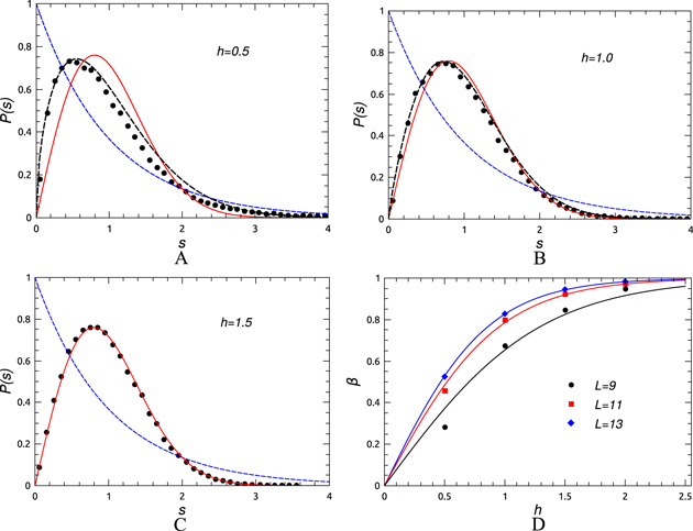
Figure 2. Level spacing distribution P(s) for the 3D non-interacting disordered model ( ) for L = 13 and for (A) h = 0.5, (B) h = 1.0 and (C) h = 1.5. The blue and black dashed lines are fits to the Poissonian and Brody distribution respectively and the red solid line to the GOE distribution. (D) The variation of β with h fit to the function
  for
for  .
.
Download figure:
Standard image High-resolution image3.2. Poissonian to GUE
We can obtain a Poisson-GUE crossover only for Model I since for Model II, the on site random potential is spin independent and does not break time reversal symmetry. In the case of Model I, if we switch on h and  both simultaneously or while keeping t, V,
  at some finite value increase h slowly, we see that P(s) changes from Poissonian to GUE as shown in figure 3. For
  and h = 0, the model is not integrable in the usual sense; it still displays Poissonian level spacing statistics as can be seen in figure 3 (it is quasi-integrable). Values of P(s) for level spacing distributions intermediate to Poissonian and GUE can be fit to a Brody form like in the previous case but this time given by

where ![$a={{(\Gamma [\frac{1+2\beta }{1+\beta }])}^{-1-\beta }}$](https://content.cld.iop.org/journals/1367-2630/16/9/093016/revision1/njp499728ieqn46.gif) .
.  for Poissonian (GUE) level spacing distributions. Again, like in the previous case we have plotted β as a function of h and fit to the function
  to obtain the crossover value of disorder strength for different system sizes.
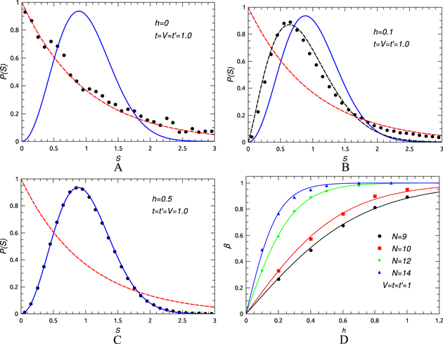
Figure 3. For Model I, the change in level spacing distribution from Poissonian to GUE for N = 14 (at half filling) for  for (A) h = 0, (B) h = 0.1 and (C) h = 0.5. The red and black dashed lines are fit to the Poissonian and Brody distributions respectively and the solid line is to GUE. (D) The variation of the parameter β as a function of h for N = 9, 10, 12, 14 and fit to the function
  .
.
Download figure:
Standard image High-resolution image3.3. GOE to GUE
As mentioned earlier time reversal symmetry is preserved in model II, hence the GOE to GUE crossover cannot be observed in it. However for model I, as shown in figure 4, keeping h fixed at some finite value (taken to be  ) and
) and  such that the GOE distribution is observed, we can easily obtain the GOE to GUE crossover by increasing
  . In this crossover region, P(s) obeys the following Brody-like one parameter functional form

where ![$c=\Gamma [1+\beta /2]$](https://content.cld.iop.org/journals/1367-2630/16/9/093016/revision1/njp499728ieqn54.gif) and
and ![$d=\Gamma [(\beta +1)/2]$](https://content.cld.iop.org/journals/1367-2630/16/9/093016/revision1/njp499728ieqn55.gif) . β changes from 1 (GOE) to 2 (GUE) as we increase
. β changes from 1 (GOE) to 2 (GUE) as we increase  . As for the previous cases, plotting β as a function of
  and fitting to
  , we calculate the crossover value of the time reversal symmetry breaking parameter (here
  ) for different system sizes as shown in figure 4.
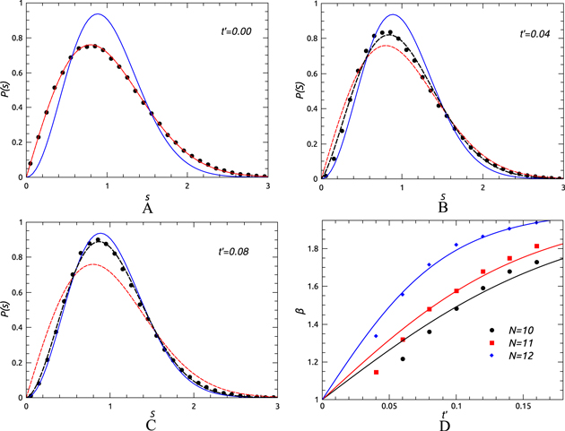
Figure 4. The change in level spacing distribution for model I showing a crossover from GOE to GUE for  (at half filling) with
  and V = 2 and h = 4 for (A)
  , (B)
, (B)  and (C)
  . The red and black dashed lines are fit to the GOE and Brody distribution and the solid blue line to GUE. (B) The variation of the parameter β with increasing
  for
for  for model I where
  , V = 2 and h = 4 and fit to the function :
 .
.
Download figure:
Standard image High-resolution image3.4. Poissonian to GSE
For model II increasing on site disorder strength (h) and SOC parameter (μ) simultaneously (here we have always assumed  a crossover from Poissonian to GSE level statistics can be obtained as shown in figure 5. Once again P(s) is fit to a Brody form
where ![$a=\frac{\Gamma [\frac{2+4\beta }{1+\beta }]}{\Gamma [\frac{1+4\beta }{1+\beta }]}$](https://content.cld.iop.org/journals/1367-2630/16/9/093016/revision1/njp499728ieqn70.gif) . One can see a crossover from Poissonian to GSE level spacing statistics as one changes β from 0 to 1. Once again β is plotted as a function of h (or μ) and fit to the function
. One can see a crossover from Poissonian to GSE level spacing statistics as one changes β from 0 to 1. Once again β is plotted as a function of h (or μ) and fit to the function  to obtain the crossover value of disorder strength for different system sizes.
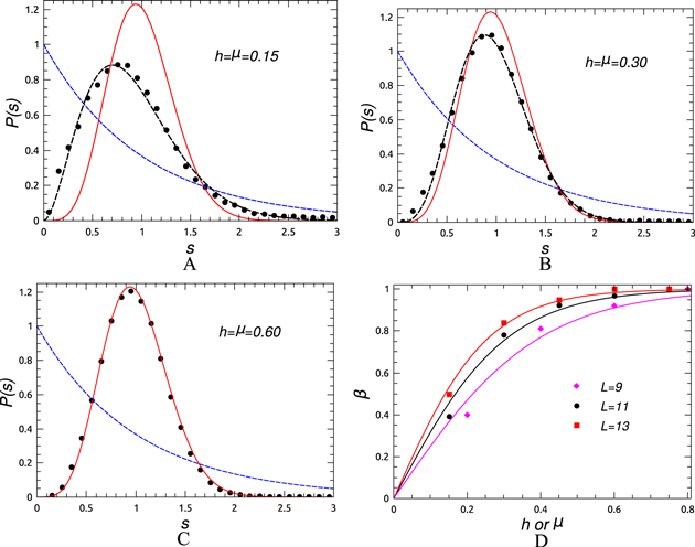
Figure 5. Level spacing distribution P(s) for the 3D non-interacting disordered model for L = 11. The values of the integrability breaking parameters are (A)  , (B)
, (B)  and (C)
  . The blue and black dashed lines are fit to the Poissonian and Brody distributions respectively and the red solid line to GSE. (D) The variation of β with h (or μ) and fit to the function
  for L = 9, 11 and 13.
Download figure:
Standard image High-resolution imageWe have also investigated the Poissonian to GSE crossover for model II for a two-dimensional square lattice. The changes in level spacing distribution and variation of β with h or  are shown in figure 6.
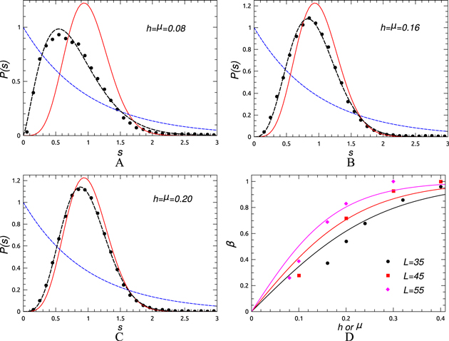
Figure 6. Level spacing distribution P(s) for the 2D non-interacting disordered model for L = 55. The values of the integrability breaking parameters are (A)  , (B)
, (B)  and (C)
  . The blue and black dashed lines are fits to the Poisson and Brody distribution respectively and the red solid line to GSE. (D) The variation of β with h (or μ) and fit to the function
  for L = 35, 45 and 55.
Download figure:
Standard image High-resolution image3.5. GOE to GSE
In the case of Model II if we set the SOC strength μ to zero and on site disorder h to a finite value (here  , the level spacing distribution will be GOE. Increasing μ, we can break spin rotation symmetry and which will cause a GOE to GSE crossover as observed in figure 7. The Brody distribution in this case is the same as in equation (11) except that β can take any value between 1 (GOE) to 4 (GSE). The variation of β with μ is fit to the function
  to calculate the crossover value of μ for different system sizes.
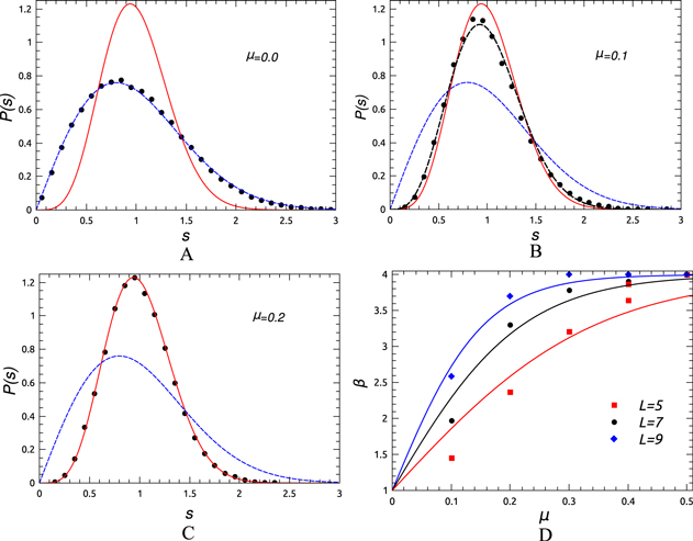
Figure 7. Level spacing distribution P(s) for the 3D non-interacting disordered model for L = 11. The values of the spin-rotation symmetry breaking parameter are (A)  , (B)
, (B)  and (C)
  . The blue and black dashed lines are fit to the GOE and Brody distributions respectively and the red solid line to GSE. (D) The variation of β with μ and fit to the function :
 for L = 5, 7 and 9.
Download figure:
Standard image High-resolution image4. Results and discussion
We now summarize the results of our calculations. For Model I, we have found that the scale of the perturbation that causes a crossover from Poissonian to GOE and GUE level statistics goes to zero with increase of system size as a power law with exponent 3 but for a GOE to GUE crossover the perturbation goes to zero as a power law with exponent 4 (figure 8). We also obtain the exponent 3 for the Poisson to GOE crossover for the interacting 1D system without disorder [22].
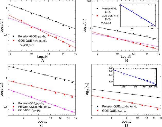
Figure 8. Crossover values (pcr) are plotted with system size on a log–log scale. For the one-dimensional interacting model the exponent for the Poissonian to GOE and GOE to GUE crossovers are respectively 3 and 4. The dashed line is the best fit to the data with slope 3 for the GOE to GUE crossover. In the inset the value of the perturbation that causes the Poissonian–GUE crossover plotted against system size and the solid line corresponds to slope 3 when (A)  ,V = 2 and (B)
  . For the non-interacting 3D disordered model (C) the perturbation causing the Poissonian–GOE and Poissonian–GSE scales as
  and the one causing the GOE to GSE crossover scale as
  , (D) the perturbation causing the Poissonian–GUE and GOE–GUE crossovers scale as
  and
and  respectively. In the inset, the perturbation causing the Poissonian–GSE crossover for the 2D model scales as
  with system size.
Download figure:
Standard image High-resolution image
For Model II, we have observed that the integrability breaking parameter which is responsible for the Poissonian to GOE/GSE crossover goes to zero as a power law with exponent 1 and for the GOE to GSE crossover this exponent becomes 3/2 (figure 8).
We have also studied a different version of Model II to investigate the Poisson to GUE and GOE to GUE crossovers. Here, we have taken the nearest neighbor hopping matrix Vij to have the following form

This model breaks time reversal symmetry. Increasing μ and h simultaneously we have observed a Poissonian–GUE crossover and then setting h = 4 and increasing μ, a GOE to GUE crossover. The exponents of the power law scaling of the crossover value of the perturbation are 1 and 3/2 for the Poissonian–GUE and GOE–GUE cases respectively.
Why do we obtain the same exponent for the Poissonian to GUE and Poissonian to GSE crossovers as we do for Poissonian to GOE? A possible answer is that the Poissonian to GUE and Poissonian to GSE crossovers can be thought of as a crossover first from Poissonian to GOE, which introduces level repulsion and then a crossover from GOE to GUE and GSE through the breaking of additional symmetries (time reversal for GOE–GUE and spin rotation invariance for GOE–GSE). For this interpretation to be correct, the fall off of the crossover value with system size for GOE–GUE and GOE–GSE has to be faster than for Poissonian–GOE. This is indeed the case for all the cases we have considered as can be seen from figure 8.
A second important question is why the Poissonian–GOE/GUE/GSE crossover scaling exponents are different for the two different models. The reason does not seem to be that the models have different dimensionality. For instance, the Poissonian–GSE crossover for Model II is the same in both two and three dimensions. We conjecture that this difference can be attributed to the fact that Model I contains interactions among the elementary degrees of freedom while Model II does not. This has a bearing on the integrable limits of these models as well in that the elementary degrees of freedom are correlated even in the integrable limit of Model I and not Model II. This difference could well be responsible for the different exponents in the two models. To further investigate this and also the role of dimensionality, it would be desirable to obtain crossovers among all the different categories of ensembles in different dimensions. However, it is not possible for us to realize a GOE phase in the non-interacting model in two dimensions owing to the fact that localization becomes operative in the absence of SOC and time reversal breaking in two dimensions. On the other hand, it is difficult to study Model I in more than one dimension since the presence of interactions greatly reduces the system sizes we can study in higher dimensions. A through investigation of the effect of interactions and dimensionality on the crossovers among different ensembles will require a study of more models which we will defer to a later work.
5. Conclusions
We have investigated the finite scaling of perturbations which cause crossovers among different random matrix ensembles in two different models: a one-dimensional model of interacting hard-core bosons (or equivalently spin 1/2) objects and a disordered model of non-interacting particles with disorder and SOC. Obtaining the level spacing distribution using numerical exact diagonalization, we have found that the scaling is a power law for crossovers among all the different ensembles (Poissonian, GOE, GUE and GSE) that can be realized in these models and obtained the corresponding exponents (see table 5). We find that the scaling from Poissonian to any of the other ensembles is dominated by the Poissonian–GOE crossover which introduces level repulsion while the symmetry breaking that causes the GOE–GUE and GOE–GSE crossovers is a sub-dominant effect. We also conjecture that there is a difference in the scaling depnding on whether the elementary degrees of freedom interact or not.
Table 1. Values of the exponent associated with the crossover among different random matrix ensembles in the presence and absence of interaction
| Ensembles | Crossover exponent | Interactions |
|---|---|---|
| Poissonian–GOE | 3 | Yes |
| Poissonian–GUE | 3 | Yes |
| GOE–GUE | 4 | Yes |
| Poissonian–GOE | 1 | No |
| Poissonian–GUE | 1 | No |
| Poissonian–GSE | 1 | No |
| GOE–GUE | 3/2 | No |
| GOE–GSE | 3/2 | No |
Acknowledgments
The authors would like to acknowledge many useful discussions with S Ramaswamy. SM thanks the Department of Science and Technology, Government of India. RM thanks Tapan Mishra for discussions and acknowledges support from the UGC Fellowship.