


Abstract
Via computer simulations, we investigate the linear and nonlinear viscoelastic response of polymer grafted nanoparticle networks subject to oscillatory shear at different amplitudes and frequencies. The individual nanoparticles are composed of a rigid spherical core and a corona of grafted polymers that encompass reactive end groups. With the overlap of the coronas on adjacent particles, the reactive end groups form permanent or labile bonds, and thus form a 'dual cross-linked' network. The existing labile bonds between particles can break and reform depending on the bond rupture rate, extent of deformation and the frequency of oscillation. We study how the viscoelastic behavior of the material depends on the energy of the labile bonds and identify the network characteristics that give rise to the observed viscoelastic response. We observe that with an increase in labile bond energy, the storage modulus increases while the loss modulus shows a more complex response depending on the labile bond energy. Specifically, in the case of the samples with the weaker labile bonds, the loss modulus increases monotonically, while for the samples with the stronger labile bonds, the loss modulus exhibits a minimum with an increase in frequency. We show that an increase in the storage modulus corresponds to an enhancement in the average number of bonds in the samples and the characteristics of the loss modulus depend on both the bond kinetics and the mobility of the particles in the network. Furthermore, we determine that the effective contribution of the bonds to the storage modulus decreases with increase in strain amplitude. In particular, while bond formation at small amplitude drives an increase in storage modulus, at large amplitudes it promotes clustering and formation of voids leading to strain softening. Our simulations provide a mesoscopic picture of how the nature of labile bonds affects the performance of cross-linked polymer-grafted nanoparticle networks.
Export citation and abstract BibTeX RIS

Content from this work may be used under the terms of the Creative Commons Attribution 3.0 licence. Any further distribution of this work must maintain attribution to the author(s) and the title of the work, journal citation and DOI.
1. Introduction
Polymer-grafted nanoparticle (PGN) networks are a relatively new class of materials [1–4] composed of nanoparticles that are decorated with long, end-grafted polymers. The free ends of the grafted polymer 'arms' encompass reactive groups, which bind to reactive groups on neighboring PGNs and thereby interconnect the nanoparticles into an extensive network. These nanoparticle networks have the dual advantage of being inorganic-rich and due to the interconnecting polymer chains, being relatively 'fluidic' (encompassing a relatively low  ). Inorganic-rich materials are vital for their superior opto-electronic and mechanical behavior, while the low
  could permit these materials to be processed at ambient temperatures through the application of external forces [5]. The presence of solvent within the network further facilitates the chains' motion, and thus makes these composites ideal candidates for low-temperature processing via applied force.
Using computational modeling, our aim is to determine the response of such PGN networks to mechanical deformations and thus, gain insight into factors that can affect the materials' ability to be dynamically reconfigured. We anticipate that the interlinking, swollen polymers impart the composite with sufficient flexibility (fluidity) that the material could be deformed and reconfigured without undergoing catastrophic failure. Via our recently developed computational approach, we have in fact shown that the PGN networks can withstand significant tensile deformation when the particles are cross-linked by both strong bonds, which break irreversibly, and weaker labile bonds, which are readily broken and reformed. We refer to these systems as 'dual cross-linked' PGN networks (see figure 1). Notably, the stronger ('permanent') bonds formed a 'backbone' that provided structural integrity and strength [2–4], while the labile bonds enabled broken interconnections to be re-made and hence, permitted re-shuffling of the bonds in the network. Acting in concert, these two types of bonding interactions led to hybrid materials that exhibited pronounced self-healing behavior, even after multiple cycles of mechanical deformation [3]. Furthermore, by optimizing the energies of the labile bonds and fraction of permanent bonds, we could significantly improve the material's toughness and the rejuvenation of its structural integrity [3].

Figure 1. Hierarchy of interactions in a network of dual cross-linked polymer grafted nanoparticles (PGNs). The grafted polymer chains contain reactive end groups, which interact to form labile or permanent bonds. At the bond-scale a force sensitive energy barrier separates the bound and the free states and thus, the model captures phenomena on the scale of bond formation (and rupture). At the nanoscopic scale, each spherical nanoparticle is represented by a rigid core that encompasses a corona of grafted chains. The overlapping of the coronas on neighboring particles enables the formation of multiple bonds between the nanoparticles. Finally, via the interactions between the PGNs and formation of bonds, the coated nanoparticles form an extended mesoscopic network.
Download figure:
Standard image High-resolution imageThis dual cross-linking might provide useful benefits when the PGN networks are subjected not only to tensile, but also more complex forms of deformation. Here, we extend our studies to determine the response of the dual cross-linked PGN networks to oscillatory shear. In particular, we now formulate a procedure for applying a strain-controlled oscillatory shear to a dual cross-linked PGN network and determine the resulting mechanical response at varying strain amplitudes and frequency of oscillation. We specifically calculate both the elasticity and dissipation of energy that characterize the PGN network under the imposed shear. Through these studies, we can relate the inherent interactions between the particles and shear response of the material in both the linear and nonlinear regimes. Moreover, we can predict effective reconfiguration conditions by pinpointing regions in parameter space that permit deformation of the material without disrupting its structural and mechanical integrity. Below, we first provide the details of our multi-component model. Next, we describe the behavior of the system in the linear regime and then analyze the performance of the material in the nonlinear regime.
2. Methodology
Our system consists of a concentrated solution of PGNs, which are cross-linked by a combination of strong or 'permanent' bonds and labile bonds to form an extended network (see figure 1). The rigid core of each nanoparticle has a radius  . The grafted polymers form a corona of stretchable chains around the nanoparticles; the thickness of this corona is given by
  . In the ensuing studies, all the length scales in the system are given with respect to the core radius
  and hence, we consider a PGN of core radius unity and a corona thickness
  .
.
The interaction between two PGNs is modeled through a sum of interaction potentials and is given by  . The first term characterizes the repulsive interactions between the coated nanoparticles and is given by [2, 6, 7]:
Here,  is the number of arms and
  is the range of the potential. The range of this repulsive potential is related to the diameter of the last blob in the Daoud−Cotton model [7, 8] and is given by
  .
.
The second term in the potential,  , describes the attractive cohesive interaction between the coated particles. This term is chosen to be a constant for small values of R, the separation between the particles, but balances the repulsion at the edges of the corona in order to allow for the overlap between neighboring coronas [2, 9]. Hence, this term is written as:

where C is an energy scale, and A and B are length scales that determine the respective location and width of the attractive well in the potential.
The final term in the potential,  , describes the attractive interaction between particles that are linked by the bonded polymer arms. The attractive force acting between the two bonded particles is given by the following equation:

where  is the number of bonds formed between the given pair of particles and
  is the spring constant, which increases progressively with the chain end-to-end distance
  [2]. The stiffening of the chain is described by the following equation obtained for a worm-like chain [10]:

In the above equation,  is the contour length of the chain formed by bonding two corona arms of length
  .
.
The value of  in equation (3) depends on the extent of overlap between the coronas of the nanoparticles and on the kinetics of bond formation and rupture
  [2]. The evolution equation for the number of bonds can be written as
  [2]:
[2]:

where  is the probability of contact of two chain ends,
  corresponds to the maximum number of bonds that can be formed between two nanoparticles, and
  and
and  are the respective rupture and formation rates at the individual bond level. The probability of contact,
  , is determined by integrating the product of the individual free-end distributions in each corona over the volume of overlap of the PGNs
  [2]. The parameter
  is estimated from purely geometric considerations by making the simplifying assumption that there is negligible distortion of the coronas.
We use the Bell model [11–14] to describe the rupture and re-formation of bonds between the polymer arms due to thermal fluctuations. In accordance with the Bell model, the rupture rate,  , is an exponential function of the force applied to the bond and is given by
  , where
  is the rupture rate in the zero force limit, which depends on the energy barrier
  separating the bound and the free states. For reversible bond formation in the zero force limit, the ratio of the formation to rupture rate is given by
  [12, 13]. In general, the rate constant of bond formation decreases under an applied force [14]. For the sake of simplicity, however, we neglect the dependence of the rate constant of bond formation on force and consider it to be constant,
  [2]. Only the labile bonds can reform after breaking; the permanent bonds can only break. In the following section, we refer to the set of bonded arms as a link; in other words, each link in the network encompasses multiple bonds.
The dynamics of the system is assumed to be in the over-damped regime, with the motion of each particle given by the equation  , where
  is the mobility and
  is the total force on the polymer grafted particle. The simulations are performed off-lattice. The total force acting on a particle can be written as
  , where
  is the external force acting on the edge particles of the particle array (see figure 1). This equation is solved numerically in two steps since the polymer spring force (within the expression for
  ) in the dynamic equation depends on the number of bonds between particles and consequently, on the evolution of the chemical kinetics given by equation (5). In the first step, we determine the number of bonds at any given time,
  , by numerically evolving the unsteady state kinetics, equation (5), through an explicit Euler scheme with a time step of
  , where
  is the unit of time in the simulation (see table 1). The numerical evolution of equation (5) yields a real number, whereas the number of bonds
  should take discrete integer values. In order to determine the integer value, we compare the fractional part of the numerical result,
  , with a random number
  distributed uniformly between 0 and 1. If
  , then we truncate the result; otherwise, we increment the integer part of the result by 1. In the second step, we use this value for the number of bonds to calculate the spring force (see equation (3)) in the dynamic equation and numerically integrate the resulting equation using a fourth-order Runge–Kutta algorithm with a time step of
  .
.
Table 1. Parameters used in the simulations.
| Dimensional units | |||
|---|---|---|---|
| Nanoparticle radius |
 = 50 nm = 50 nm |
||
Time, 
|
 = 1.41 × 10⁻² s = 1.41 × 10⁻² s |
||
Force, 
|
 = 2.98 pN = 2.98 pN |
||
| Bond parameters | Weaker labile bond | Stronger labile bond | Permanent bond |
Bond energy, 
|

|

|

|
Rupture rate at zero force, 
|

|

|

|
Formation rate, 
|

|
0 | |
Bond sensitivity, 
|

|
||
| Characteristics of polymer grafted nanoparticle (PGN) | Corona thickness 
|
||
Kuhn length, 
|
1 nm | ||
Number of grafted arms, 
|
156 | ||
Arm contour length, 
|

|
||
Chain spring constant, 
|

|
||
Repulsion parameter, 
|

|
||
Cohesion parameters, 
|

|
||

|

|
||

|

|
||
Mobility of PGN, 
|

|
||
In the studies described below, we consider a particle of core radius  nm with
  polymer chains grafted onto its surface and specify the corona of grafted arms to have a thickness of
  . The value of
  is used to determine the strength of repulsion and extent of bond formation between any two interacting particles through equation (1) and equation (5), respectively. The cohesive interaction in equation (2) with
  ,
,  and
and  counters the repulsive forces at the corona edge. The equilibrium overlap between two particles is such that for the labile bond energy of
  , the particles are separated by a center-to-center distance of
  (corresponding to
  overlap) and are connected by approximately seven bonds. The mobility of particle,
  , is computed as the inverse of the Stokes drag,
 ![$\mu ={{[6\pi \eta \;{{r}_{0}}(1+q)]}^{-1}}$](https://content.cld.iop.org/journals/1367-2630/16/7/075009/revision1/njp497074ieqn93.gif) , on a particle of radius
, on a particle of radius  in a viscous fluid of viscosity
  (viscosity of glycerol). For convenience, all the parameters used in the simulations are collected in table 1. In simulating the bond kinetics, we fix the bond energy of the permanent links to be
  and examine two cases of labile bond energies:
  and
and  .
.
Each sample in the simulations is composed of  particles, which are initially arranged in 13 rows, with 14 particles in each row (see figure 1). The initial state of the system is generated using the following five-step procedure. In the first step, the nanoparticles are placed in an array such that their centers are separated by a horizontal spacing of
  and a vertical spacing of
  , with a horizontal offset position of
  between adjacent rows. In the second step, we hold the sample in the initial configuration for 4000
  units of time to allow for the formation of the labile bonds. In the third step, we equilibrate the sample for a time 6000
  , during which the stressed labile bonds are broken and new bonds are formed between the adjacent PGNs according to equation (5). Note that the particles rearrange their positions in continuous space because the simulations are performed off-lattice. In the fourth step, we introduce the permanent bonds into the system. In this step, a certain number of already established labile bonds are converted randomly to permanent ones; as a result, each pair of neighboring particles has an average of
  permanent bonds. Finally, in the fifth step, the resultant sample composed of a dual cross-linked network of permanent and labile bonds is equilibrated for
  time steps, with the breakage and formation of the labile bonds being allowed.
In order to impose an oscillatory shear deformation, the coordinates of the particles at the lower edge of the sample are fixed in space, and each particle at the top edge is moved in the  direction at small increments so that the time-dependent displacement,
  , is
, is  . Here,
  is the height of the sample, which is kept constant in the course of simulations,
  is the amplitude of the shear and
  is the frequency of the oscillations. To minimize the finite size effects, the shear displacements are also imposed on the particles at the left and right edges of the sample. It is worth recalling that the simulations are performed off-lattice, so that the particles in the bulk of the network move in continuous space in the course of the shear deformation. The
  component of the force,
  , that acts on the particles at the top layer (shear force) is recorded as a function of time
  at various values of
  and
and  . We plot Lissajous curves showing the behavior of
  , the force in the
  direction as a function of the time-dependent displacement,
  . These curves are generated and analyzed to characterize the elasticity and dissipation in the system as functions of
  . At small shear amplitudes (the linear regime), the elasticity and dissipation are described by the storage modulus,
  , and the loss modulus
  , respectively. Namely,
  is the Fourier component of the shear force that is in-phase with the shear strain, and is determined from the tilt of the Lissajous curve. In turn,
  is the Fourier component of the shear stress that exhibits a phase difference of
  from the shear strain, and is determined from the area bounded by the Lissajous curve. At large shear amplitudes (the nonlinear regime), the Lissajous curves provide the measures of elasticity and dissipation that are generalizations of
  and
and  , respectively.
Using the approach described above, we study the viscoelastic response of the material to an applied oscillatory shear deformation characterized by  . The shear strain amplitude
  is calculated as the ratio of the shear deformation of the sample to its height in the undeformed state, i.e., in the state achieved in the course of the sample preparation described above. The shear amplitude and angular frequency of oscillations are varied within the respective ranges of
  and
and  rad s−1. The frequency range is chosen to be sufficiently wide that it allows us to study the effect of altering the energy of the labile bonds on the viscoelastic response of the network. Specifically, the characteristic frequencies,
  , which are associated with the labile bonds at the energies of
  and
and  , are
, are  rad s−1 and
  rad s−1, respectively. The force response of the network to the applied shear is analyzed in the cases of linear and nonlinear deformations. Eight independent runs are performed on the samples for each set of chosen parameters in order to quantify the dynamic response.
3. Results and discussion
3.1. Linear viscoelastic behavior at small shear strain
We first consider the dynamic response of the system to oscillatory shear deformations for the case of a small amplitude of the applied shear, setting  . In figure 2, we plot the shear force and average number of bonds in the network as functions of the shear strain, and show that the response of the network depends on both the energy of the labile bonds and frequency of oscillation. In particular, depending on the values of
  and
and  , the force–strain Lissajous curves form a straight line (see figures 2(a) and (b)) or an ellipse (see figures 2(b)–(d)). The Lissajous curves indicate that the PGN network exhibits linear viscoelastic behavior at
  . The tilt of an ellipse (slope of a straight line) is proportional to the storage modulus
  , which characterizes the elasticity of the system. The width of an ellipse is proportional to the loss modulus
  , which is a measure of the dissipation in the system due to a lag between the applied strain and the resulting force.

Figure 2. Shear force and average number of bonds in a network as a function of shear strain for two different labile bond energies  = 1:33 (blue curves) and 2:37 (red curves) and increasing frequency of oscillations
  = 3 × 10⁻³, 3 × 10⁻², 3 × 10⁻¹, 3 × 100. (a)–(d) Shear force (
 ) versus strain (
 ) curves. (e)–(h) Number of labile bonds per particle
  versus strain (
 ) curves.
Download figure:
Standard image High-resolution imageAt a given frequency,  , the samples with the stronger labile bonds exhibit a larger tilt of the force–strain Lissajous curves, indicating that they have higher storage moduli (see figures 2(a)–(d)). The latter behavior can be attributed to the increase in the number of bonds with the increase in bond strength (see figures 2(e)–(h)). Furthermore, figure 2 shows that for both the weaker and stronger labile bonds, the number of labile bonds and the storage moduli (tilt of the Lissajous curves) increase with an increase in the frequency of oscillation,
  . Finally, the dissipation in the system is seen to depend on
  , as indicated by the variations in the width of the Lissajous curves in figures 2(a)–(d).
The storage and loss moduli as functions of the oscillation frequency (at the shear amplitude of  ) are shown in figures 3(a) and (b), respectively. To calculate the moduli
  and
and  , we first determine the amplitude of the force,
  , and the phase difference,
  , by fitting the shear force
  , which is obtained from the strain-controlled simulations at
  , to the equation
  . Then, the moduli are found as:


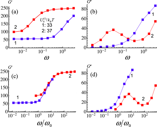
Figure 3. Storage and loss moduli, respectively at the shear amplitude of  for two different labile bond energies
  = 1:33 (blue symbols and curves) and 2:37 (red symbols and curves). (a)–(b) Storage
  and loss
  moduli as a function of oscillation frequency
  . (c)–(d) Storage
  and loss
  moduli as a function of normalized oscillation frequency
  .
.
Download figure:
Standard image High-resolution imageThe storage and loss moduli could also be determined directly from the Lissajous curves [15].
The storage modulus of the network shows two distinct features. First, as noted above,  increases with an increase in the energy of the labile bonds
  , so that it is consistently greater at
  than at
  (see figure 3(a)). Second,
  exhibits a transition from a lower plateau to a higher plateau value with an increase in frequency for both the
  considered here. The increase in
  shifts the transition to the lower frequencies (figure 3(a)). On the other hand, the loss modulus
  as a function of
  exhibits distinctly different behavior at the weaker and stronger labile bonds (see figure 3(b)). Namely,
  increases monotonically at
  (curve 1 in figure 3(b)), whereas at
  , the loss modulus exhibits a peak (see curve 2 figure 3(b)). The latter peak is located within the frequency range where the storage modulus of the system,
  , exhibits a transition between the two plateaus (compare curves 2 in figures 3(a) and (b)).
It is instructive to plot the moduli  and
and  as functions of the normalized frequency
  (see figures 3(c) and (d), respectively), where
  is the characteristic frequency, which depends on the energy of labile bonds
  through the rupture rate constant,
  . The storage modulus
  as a function of
  shows the same behavior for the networks containing the weaker and stronger labile bonds. Namely,
  exhibits a lower plateau regime at
  , a higher plateau regime at
  , and a smooth transition between the latter two regimes at
  . Figure 3(c) indicates, therefore, that at low strain amplitudes, the network elasticity (storage modulus) as a function of frequency is controlled by the rupture rate
  of the labile bonds. The latter conclusion cannot be made, however, for the frequency-dependent dissipation in the network. Figure 3(d) shows that the loss modulus
  as a function of
  behaves quite differently at
  and
and  . The reason for the observed behavior of
  is associated with dissipation due to the particle–solvent friction, which does not depend on the energy of the labile bonds and is linearly proportional to
  .
.
The effect of the particle–solvent friction is demonstrated in figure 4, where we plot the storage and loss moduli as functions of  at three values of the mobility, which is inversely proportional to friction. Figure 4(a) shows that the storage modulus
  is unaffected by the variations in the value of the mobility. In contrast, the loss modulus
  exhibits notable changes as the mobility is varied. Within the high frequency region (see figure 4(b)),
  decreases with an increase in the mobility, i.e., with a decrease in the particle–solvent friction. Namely, the effect of friction on
  becomes noticeable at
  for both the weaker and stronger labile bonds. It is worth noting that at
  , the behavior of
  at the mobility of
  indicates the onset of a maximum (at
  ) that is not observed in the samples with lower mobility.

Figure 4. Storage and loss moduli as a function of normalized oscillation frequency  at the shear amplitude of
  for two different labile bond energies
  = 1: 33 (blue symbols and curves) and 2: 37 (red symbols and curves), and three different particle mobilities: (●)
  , (■)
, (■)  and (▼)
  . (a) Storage
  modulus, (b) loss
  modulus.
Download figure:
Standard image High-resolution imageTo gain greater insight into the simulation results, we consider a simple model, which captures all the salient features of the viscoelastic behavior arising from the dynamics of the labile bonds. In our simulations, the nanoparticles in the PGN network form a hexagonal lattice at equilibrium (as observed in recent experimental studies on a comparable system [16]). We note that the hexagonal lattice is a stable configuration and alternate initial configurations of square and face centered square lattices spontaneously transform to the hexagonal lattice during equilibration. Hence, we consider the system of three particles shown in figure 5 as a representative cell of the lattice shown in figure 1, and determine the response of this cell to a strain-controlled oscillatory shear deformation. Specifically, particles 1 and 2 are fixed in space, whereas particle 3 exhibits oscillations in the horizontal direction, as indicated in figure 5. The position of particle 3 in the vertical direction is held constant at  and the horizontal coordinate changes in time as
  , where
  and
and  are the equilibrium center-to-center distance between the particles and shear amplitude, respectively. The time-dependent distance between the particles in pairs 1–3 and 2–3 is calculated as
 ![$R(t)={{Y}_{0}}{{[1+{{({{3}^{-1/2}}\pm {{\gamma }_{0}}\;{\rm sin} \left( \omega \;t \right))}^{2}}]}^{1/2}}$](https://content.cld.iop.org/journals/1367-2630/16/7/075009/revision1/njp497074ieqn223.gif) , where the signs '+' and '−'correspond to the pairs 1–3 and 2–3, respectively. Within each pair, the dynamics of the rupture and formation of the labile bonds is described by the following master equation [17] for the probability of finding
, where the signs '+' and '−'correspond to the pairs 1–3 and 2–3, respectively. Within each pair, the dynamics of the rupture and formation of the labile bonds is described by the following master equation [17] for the probability of finding  labile bonds
  :
:

Here,  is the rate coefficient for the rupture of labile bonds defined in section 2 and
 ![${{k}_{f}}(R,n)={{[{{N}_{{\rm max} }}(R)-n]}^{2}}{{P}_{c}}(R)\;k_{0f}^{(l)}$](https://content.cld.iop.org/journals/1367-2630/16/7/075009/revision1/njp497074ieqn227.gif) is the rate coefficient for the bond formation (cf equation (5)). The probability of having no labile bonds between a pair of particles,
is the rate coefficient for the bond formation (cf equation (5)). The probability of having no labile bonds between a pair of particles,  , is found from the normalization condition to be
  . It is worth recalling that the inter-particle distance
  in equation (8) is a function of time
  (as described above).

Figure 5. Illustration of the basic three particles simulation set up. Particles 1 and 2 are fixed in space, whereas particle 3 undergoes oscillations in the horizontal direction.
Download figure:
Standard image High-resolution imageThe system of equations generated from equation (8) was truncated at  and solved numerically for the two pairs of particles using the Mathematica™ software. The model parameters used in these calculations were the same as used in the simulations of the array of particles. Upon solving equation (8), the value of attractive force between two particles due to bonded polymer arms was calculated according to equation (3) at the number of bonds
  . The latter equation means that the link consists of one permanent bond and an average number of labile bonds given by
  . Finally, the values of
  and
and  were determined using the numerical Fourier transform applied to the X component of the total force acting on particle 3.
In figures 6(a) and (b), we compare the behavior of the storage and loss moduli as functions of  for the three particle model (figure 5(a)) and for the array of particles (figure 1) at
  and
and  , and the strain amplitude
  . Only a qualitative comparison is possible since, in our simulations, the magnitudes of the calculated modulus is based on the force required to shear the array of particles and, hence, depends on the size of the array. To make these comparisons, the moduli
  and
and  were normalized by
  , which corresponds to the plateau value of the storage modulus at the lower frequencies, i.e.,
  . The normalized storage moduli obtained from the three-particle model (solid lines) and from simulations of the array of particles (symbols) are in quantitative agreement at both values of the labile bond energies considered here (see figure 6(a)). Note that the three-particle model takes into account only the processes of rupture and formation of the labile bonds between the individual pairs of PGNs. The latter result (figure 6(a)) indicates, therefore, that at low shear strains, the individual PGN pairs contribute independently to the elastic properties of the material, i.e., there are no collective effects.
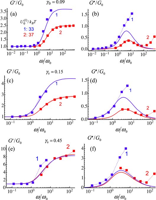
Figure 6. Comparison of the normalized storage  and loss
  moduli obtained for the three-particle model with that of the array of particles at two different labile bond energies
  = 1:33 (blue symbols and curves) and 2:37 (red symbols and curves) and three different amplitudes
  : (a), (b) 0.09, (c), (d) 0.15 and (e), (f) 0.45.
Download figure:
Standard image High-resolution imageFigure 6(b) shows the normalized loss moduli for the three-particle model (solid lines) and PGN array (symbols). For the three-particle model,  exhibits a peak at the value of
  where
where  exhibits an inflection point within the transition zone between the lower and higher plateaus (figure 6(a)). Such behavior is typical for cross-linked viscoelastic polymeric systems [18]. In networks of cross-linked PGNs, the viscoelastic behavior is caused by the rupture and formation of the labile bonds, and the dissipation is maximal when the characteristic times of shear deformation and of bond rupture are comparable
  . Notably, for
  (the stronger bond), the peak in the loss modulus for the three-particle model coincides with the peak for the PGN array (figure 6(b)), indicating the predictive ability of the simplistic three-particle model. The peak in
  at
at  is not observed for the cross-linked array of PGN because it is masked by dissipation due to the particle–solvent friction. (We will return to this figure to discuss the behavior in the nonlinear regime, which is captured by figures 6(c)–(f).)
The three-particle model served to highlight the importance of the breaking and making of labile bonds in the viscoelastic response of the system to the oscillatory shear. Figure 7 shows how the number of labile bonds depends on changes in the scaled shear frequency  for
for  . (Recall that
  depends on the rupture rate constant for the bond.) In this figure, we show the difference in number of labile bonds,
  , between each bonded pair of PGNs in the array at the maximal
  and zero
  shear strains. The variations
  are shown for three values of
  (figures 7(a)–(c)). The respective frequencies
  in figures 7(a)–(c) are the same as those in figures 2(e), (f) and (h), which show the Lissajous curves for the number of the labile bonds per particle,
  . At the lowest frequency
  (figure 7(a)), the oscillatory shear causes the greatest variation in the number of labile bonds between individual pairs of PGNs. The variation in
  decreases with an increase in the frequency of oscillation, so that at the highest frequency
  , only a few pairs of PGNs exhibit a change in the number of labile bonds in the course of deformation from
  to
to  (figure 7(c)).
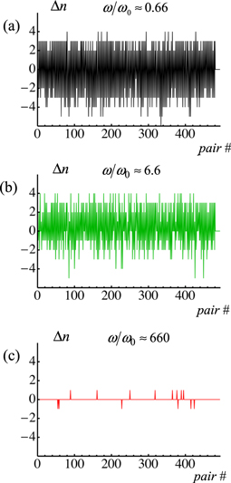
Figure 7. The difference in number of labile bonds,  , between each bonded pair of PGNs in the cross-linked array of particles at the maximal
  and zero
  shear strains at three different values of normalized oscillation frequency
  (a) 0.66, (b) 6.6 and (c) 660.
Download figure:
Standard image High-resolution imageAs noted with respect to the discussion of figure 6(b), the dissipation in the system (value of the loss modulus) reaches a maximum value when  . The rupture and formation of the labile bonds do not contribute to the loss modulus at both the lower and higher frequencies (see the solid lines in figure 6(b)), although the variations
  are drastically different at these two extremes (compare figures 7(a) and (c)). At the lower frequency, the labile bonds break and reform faster than the progression of the shear deformation. Therefore, no hysteresis is observed in the number of bonds in the system, as evident from figure 2(e) (see curve 2), and hence, there is no contribution to dissipation. In contrast, at the higher shear frequency, the rate of rupture of the labile bonds is much lower than the shear rate. The number of labile bonds does not change noticeably in the course of an oscillation cycle (see curve 2 in figure 2(h)), so again there is no contribution to dissipation. The rupture and reformation of the labile bonds contribute to the loss modulus when the bond rupture rate and shear rate are comparable, so that the number of labile bonds exhibits hysteretic behavior (see loops in curve 2 in figure 2(f)).
As demonstrated above, the viscoelastic properties of the PGN networks that are caused by rupture and formation of the labile bonds are governed by the bond rupture rate constant,  , which depends on the bond energy. The viscoelastic behavior of the PGN networks cannot, however, be considered as a result of a single relaxation process characterized by the relaxation time
 . This is evident from figure 8, which shows Cole−Cole plots for the PGN networks with labile bonds of energy
  (plot 1) and
  (plot 2). In a Cole–Cole plot, the properly normalized frequency-dependent loss and storage moduli are plotted against each other. The normalization is performed as indicated in figure 8, where
  is the low frequency plateau value of the storage modulus, and
  is the difference between the high and low frequency plateau values of
  . It is known that if viscoelastic relaxation is characterized by a single relaxation time, then the Cole–Cole plot forms a semi-circle indicated by curve 3 (dashed line) in figure 8 [19, 20]. In contrast, figure 8 shows that the Cole–Cole plots for the viscoelastic moduli obtained from both the results of simulations (symbols) and the three-particle model (solid curves) lie well below the semicircle. The only exceptions are the symbols on the right that correspond to the simulations at the higher frequency of shear oscillations where the particle-solvent friction dominates (see above).

Figure 8. Cole−Cole plots for the viscoelastic moduli obtained from both the results of simulations (symbols) and the three-particle model (solid curves) at  = 1:33 (blue symbols and curves) and 2:37 (red symbols and curves). The dashed black curve is the Cole−Cole plot for a system with a single relaxation time.
Download figure:
Standard image High-resolution imageThe features of viscoelastic behavior revealed through the Cole–Cole plots (figure 8) are characteristic of rheologically complex materials, for which the stress relaxation exhibits a stretched exponential dependence on time and hence, the spectrum of relaxation times is continuous [19, 20]. The viscoelasticity of rheologically complex materials could be described in terms of the customary linear springs and dashpots only if an infinite, hierarchical system of springs and dashpots is considered [19, 20]. It is rather remarkable that the simple three-particle model, which takes into account only the breakage and formation of bonds (see figure 5 and equation (8)), is capable of reproducing the characteristic features of the rheologically complex behavior of the PGN network as seen in figure 8. Hence, we can conclude that the relaxation processes in this system are controlled mostly by the kinetics of bond rupture and formation. In order to demonstrate how the bond kinetics results in a spectrum of relaxation times, in figures 9(a)–(c) we plot the evolution of the average number of bonds,  , obtained for the three-particle model through solving equation (8) at the different values of
  indicated in the figures. The lines labelled by
  and
and  correspond to the average number of bonds between particles 1 and 3 and particles 2 and 3, respectively (see figure 5 and figures 9(a)–(c)). The values of
  and
and  exhibit step-wise variations at the frequencies of
  and 6.6 (see figures 9(a), (b), respectively), and saw-tooth kinetics is observed at the higher frequency of
  (figure 9(c)). Such a highly nonharmonic response of the average numbers of bonds
  and
and  to the sinusoidal shear deformations cannot be represented by a combination of a few Fourier harmonics. As the attractive force between two particles is proportional to the average number of bonds, the stress relaxation exhibits a spectrum of relaxation times, which is a characteristic feature of the rheologically complex behavior.
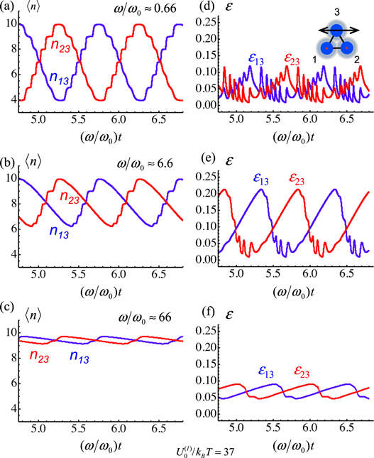
Figure 9. The average number of labile bonds,  , between particles 1 and 3 and particles 2 and 3 as a function of dimensionless time at three different values of normalized oscillation frequency
  (a) 0.66, (b) 6.6 and (c) 66. The fluctuations in the average number of labile bonds,
  , between particles 1 and 3 and particles 2 and 3 as a function of dimensionless time at three different values of normalized oscillation frequency
  (d) 0.66, (e) 6.6 and (f) 66.
Download figure:
Standard image High-resolution imageIt is important to note that the average numbers of bonds  and
and  shown in figures 9(a)–(c) are obtained by solving the master equation, equation (8), and in this way, we account for stochastic effects. The contribution of the stochastic effects can be estimated by calculating the value of relative deviation
  ; the stochastic effects can be neglected at
  . Figures 9(d)–(f) show the time-dependent values of
  calculated for the pairs of particles 1–3 and 2–3 and denoted as
  and
and  , respectively, at the same frequencies of shear oscillation as in figures 9(a)–(c). The stochastic effects cannot be neglected as
  at the frequencies of
  and 66 (figures 9(d) and (f), respectively), and
  at the intermediate frequency
  (figure 9(e)). It is worth noting that the frequency
  , at which the stochastic effects are especially important, corresponds to the peak in the loss modulus (see figure 6(b)).
3.2. Nonlinear behavior under large amplitude oscillatory shear
The response of the PGN networks to oscillatory shear deformations is nonlinear under sufficiently high shear amplitudes. In the nonlinear regime, the force–strain Lissajous curves deviate from the elliptical shape. Figure 10 shows Lissajous plots obtained from the simulations of the PGN network at shear frequencies of  (figures 10(a)–(c)) and 3 (figures 10(d)–(f)) and shear amplitudes from
  to 0.45. Here, we fixed the labile bond energy at
  . The shape of the Lissajous curves changes dramatically as the shear amplitude
  is increased, and that the shape distortion is more pronounced at the lower relative frequency of oscillation
  . Furthermore, the shear force (marked in gray in figure 10) exhibits noticeable fluctuations, which increase with an increase in the amplitude of shear
  .
.
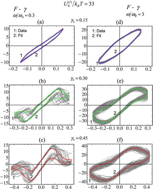
Figure 10. Lissajous plots obtained from simulations of the PGN network, which contains the labile bonds having the energy  , at the strain amplitudes from
  = 0.15, 0.30 and 0.45 and the normalized oscillation frequency
  (a)–(c) 0.3 and (d)–(f) 3.
Download figure:
Standard image High-resolution imageThe nonlinear response of the material to the large amplitude oscillatory shear (LAOS),  , can be analyzed by representing the time dependent shear force
  as a Fourier series, i.e.,

Here,  and
and  are the Fourier coefficients, which depend on the shear frequency
  and amplitude
  . It is more useful, however, to consider the force
  as a function of the instantaneous values of shear strain
  and shear strain rate
  , and then decompose
  into the elastic part
  , which depends only on the strain, and the strain rate-dependent viscous contribution
  :
:

The above decomposition can be performed in a straightforward manner if the elastic and viscous contributions are represented by Chebyshev polynomials of the first kind [21, 22]:


where  is the strain rate amplitude. The Chebyshev polynomials
  are defined by the following recursive relation [23]:

The first harmonic coefficients in the Fourier series in equation (9) provide a measure of the average (over one cycle of oscillation) values of the storage and loss moduli  and
and  , respectively, which are related to the first Chebyshev coefficients in equations (11) and (12) as follows:


To determine the average storage and loss moduli from the results of the simulations, we employ equations (10)–(12), in which the first four terms of the Chebyshev expansion (n = 1, 3, 5 and 7) are used to fit the shear force over 20 consecutive cycles of oscillation. Fitting was performed using the Mathematica™ software. The Lissajous curves obtained by the fitting procedure are shown in figure 10 by the thick colored lines. Finally, the values of  and
and  are calculated according to equations (14) and (15) followed by averaging over eight independent runs.
Figures 11(a)–(d) show the Lissajous curves obtained from the Chebyshev analysis of the shear force at various values of the strain amplitude  and scaled frequency
  . The Lissajous curves showing the average number of labile bonds versus the shear strain in the respective samples are presented in figures 11(e)–(h). The plots for
  and 3 are obtained from the results of simulations at the energy of labile bonds
  , and the plots for
  and 33 correspond to
  . The Lissajous curves in figures 11(a)–(d) clearly show that the nonlinearity of the force response to the oscillatory shear deformations (indicated by deviation of the curves from elliptical shape) increase with the strain amplitude, and are more pronounced at the lower values of
  . Notably, a strain softening is observed at low frequencies, i.e., the shear force decreases with an increase in shear strain at
  (see figures 11(a) and (b)).
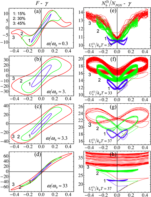
Figure 11. Lissajous curves obtained from the Chebyshev analysis of the shear force and the number of labile bonds per particle at three different values of the strain amplitude  = 0.15, 0.30 and 0.45 and increasing values of normalized oscillation frequency
  0.3, 3, 3.3 and 33. (a)–(d) Chebyshev shear force
  versus strain (
 ) curves. (e)–(h) Number of labile bonds per particle
  versus strain
  curves.
Download figure:
Standard image High-resolution imageThe number of labile bonds in the system also depends on both the amplitude  and relative frequency
  of oscillations (figures 11(e)–(h)). At
  , during a cycle of shear oscillation, the variation in the number of labile bonds increases with the shear strain amplitude
  (figure 11(e)). At a sufficiently high frequency of oscillation, an increase in
  leads to an increase in the number of labile bonds, but the number of bonds shows very little variation over an oscillation cycle (figure 11(h)). At
  ,
,  exhibits hysteretic behavior, as indicated by the looped Lissajous curves in figures 11(f) and (g), and both the average number of bonds and the range of variation increase with
  .
.
The average storage and loss moduli extracted from the results of simulations in the LAOS regime are shown in figures 12(a) and (b), respectively. Comparison of figures 3 and 12 reveals that both  and
and  for the PGN networks exhibit very similar behavior as functions of
  in the linear and nonlinear regimes. (Recall that
  depends on the energy of the labile bonds.) An increase in the shear amplitude is seen to affect mostly the average storage modulus, as
  decreases consistently with an increase in the shear amplitude (figure 12(a)). The decrease in
  is attributed to the strain softening, which occurs at the shear strains
  as discussed above. In contrast, variations in the amplitude of the strain produce very little effect on the dissipative properties of the PGN networks characterized by the average loss modulus
  , as a comparison of figures 3(d) and 12(b) shows.

Figure 12. Average (a) storage  and (b) loss
  moduli extracted from the results of simulations in the LAOS regime at three different values of the strain amplitude
  = 0.15, 0.30 and 0.45.
Download figure:
Standard image High-resolution imageTo further demonstrate the similarity in the viscoelastic response of the materials in the linear and nonlinear regimes, we compare the results of simulations for the LAOS deformations with the calculations obtained from the three-particle model (figure 5), which accurately described the linear case (figures 6(a), (b)). Figures 6(c)–(f) present the normalized average storage and loss moduli determined from the simulations (symbols) and from the model calculations (solid lines) at the strain amplitudes of  = 0.15 and 0.45. At
  = 0.15,
  obtained from the three-particle model is in a good agreement with the data from the simulations of the network (figure 6(c)), and the agreement is fairly good at the larger strain amplitude
  = 0.45 (figure 6(e)). Furthermore, similar to the linear regime, the three-particle calculations reproduce the peak observed in the loss modulus
  for the PGN network containing the stronger labile bonds (compare curves 2 in figure 6(b) and in figures 6(d), (f)). Therefore, we can conclude that the viscoelastic relaxation in the LAOS regime is governed by the same processes as in the linear case.
We now utilize the three-particle model (figure 5) to discuss the effect of strain softening observed in the LAOS regime (see figure 11(a)). Figure 13 indicates that the strain softening effect can be explained through geometric arguments. Figures 13(a) and (b) show schematically the forces acting on particle 3 in the system of three PGNs at the shear strains  and 0.45, respectively, with
  and
and  being the respective attractive and repulsive force within the pair
  ,
,  or (23). At
  , the repulsive forces acting on particle 3 within pairs 1–3 and 2–3 compensate each other, whereas the sum of the attractive forces is small but non-zero because
  due to the hysteretic behavior of the average number of bonds (figure 13(a)). With the shear deformation, the individual forces change their magnitude and direction. As seen in figure 13(b), the repulsive and attractive forces in pair 1–3 become more oriented towards the direction of shear (the horizontal direction) but decrease in magnitude. In contrast, the forces in pair 2–3 increase in magnitude, but become more oriented in the normal to the shear direction (figure 13(b)). As a result, the total force in the direction of the applied shear is small at
  as seen in figure 13(b), i.e., strain softening takes place. The shear,
  , and normal,
  , components of the force as functions of the oscillatory shear strain (the Lissajous curves) obtained for the three-particle model at
  and
and  = 0.45 are shown in figure 13(c). At
  , the magnitude of the shear force
  decreases with an increase of shear strain (curve 1), whereas the magnitude of the normal force
  continues to increase (curve 2). Notably, the three-particle model reproduces the value of shear strain at the onset of shear softening
  observed in the simulations of the crosslinked array of PGNs (as can be seen by comparing curve 3 in figure 11(a) and curve 1 in figure 13(c)).

Figure 13. Schematic of force components acting on particle 3 due to particles 1 and 2 at (a)  = 0 and (b)
  = 0.45. (c) Shear and normal force components from the three-particle model for the weak
  labile bonds system subject to large amplitude oscillation with
  = 0.45 at relative frequency of
  .
.
Download figure:
Standard image High-resolution imageFinally, it is important to note that the PGN networks could exhibit noticeable structural changes in the LAOS regime depending on the frequency of shear strain oscillation  relative to the characteristic frequency
  , which, in turn, depends on the energy of the labile bonds. Figure 14 shows snapshots of the simulations at the higher strain amplitude
  that correspond to the moments of time when the shear strain is
  = 0 and 0.45. Only labile bonds between the particles are shown in figure 14, and the number of bonds in a link is indicated by the thickness of the line. Thus, the thicker lines indicate more labile bonds in the link. Figures 14(a) and (b) show the configuration of the labile bonds at the lower relative frequency
  for the shear strain of
  = 0 and 0.45, respectively; figures 14(a) and (b) were obtained at
  . Figure 14(b) shows that at
  = 0.45, the distribution of the labile bonds is non-uniform in the system, i.e., some PGN pairs have many labile bonds between them (thick lines) and some have none (voids). Nevertheless, when
  , the particles return to the hexagonal arrangement (compare figures 1 and 14(a)) because the labile bonds rupture and reform sufficiently rapidly at the given frequency of oscillation
  .
.
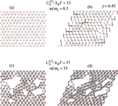
Figure 14. Snapshots of the simulations at the highest strain amplitude  that corresponds to the moments of time when the shear strain is
  = 0 and 0.45 at (a), (b)
  and ω/ω0 ≈ 0.3 and (c), (d)
  and ω/ω0 ≈ 33. Only labile bonds between the particles are shown and the number of bonds in a link is coded by thickness of the line.
Download figure:
Standard image High-resolution imageThe PGN network exhibits quite different structural features in the opposite case of  , as shown in figures 14(c) and (d) for the configuration of the labile bonds at
  ;
;  in figures 14(c) and (d). Since the newly formed labile bonds do not have enough time to rupture during one cycle of oscillation, the particles start aggregating owing to the increased attractive forces, and the latter leads to the formation of cavities after several cycles of deformation (figures 14(c) and (d)).
Note that in figure 14, the opposite cases of lower ( in figures 14(a) and (b)) and higher (
 in figures 14(c) and (d)) relative frequency were obtained by varying both the frequency
  and the energy of the labile bonds
  . At a given value of
  , the configurations of labile bonds look similar in the cases of the weaker and stronger labile bonds (not shown here but see the discussion below).
In the LAOS regime, the local distribution of shear strain within a deformed PGN network becomes spatially non-uniform if the relative frequency  is sufficiently low. The value of shear strain in the vicinity of a particle is calculated by averaging the shear strains determined in the two triangular elements to which the particle belongs in the undeformed state. In figure 15(a), particle 1 belongs to the elements (123) and (145) formed by the neighboring particles 1, 2, 3 and 1, 4, 5, respectively. The shear strains in the two elements are determined as
  and
and  , where
  are the coordinates of the particle
 . Then, the shear strain localized at the particle 1 is calculated as
  . Figure 15(b) shows the histograms of the local shear strain in the PGN network having the labile bonds of the energy
  obtained in the LAOS regime at the relative frequencies of
  (top histogram) and 0.3 (bottom histogram) and the strain amplitude
  . The histograms correspond to the moments of time when the shear strain is maximal
  . At the higher frequency of
  , the distribution of shear strain is bell-shaped and centered around the value of the imposed strain
  (figure 15(b)). In contrast, at the lower frequency of
  , the distribution of strain is rather featureless but remarkably wide, revealing the presence of areas where the local shear strain is lower
  and higher
  than the imposed strain (figure 15(b)). The observed non-uniformity of the local strains is evidence of local rearrangements of particles that occur because the labile bonds between the neighboring PGNs break in the course of deformation if the deformation is sufficiently slow (low frequency). If the deformation is fast (high frequency), the breakage of labile bonds during deformation is less prominent so the shear strain is distributed more uniformly within the sample. Note that this is the relative frequency of oscillations
  that controls the effect. It is seen in figures 15(c) and (d) that the distributions of strain in the samples having weaker
  and stronger
  labile bonds are quite similar if the relative frequency of oscillations is the same (
 and 33 in figures 15(c) and (d), respectively).
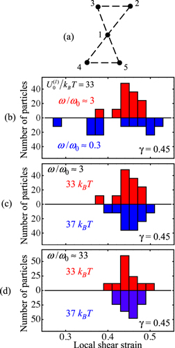
Figure 15. (a) Schematic of shear deformation in the vicinity of a particle belonging to two triangular elements of the PGN network. Histograms of the local shear strain obtained in the LAOS regime at the moments of time when the shear strain is maximal  in the PGN network (b) with labile bonds of energy
  at the relative frequencies of
  (top histogram) and 0.3 (bottom histogram), (c) with weak
  (top histogram) and strong
  (bottom histogram) labile bonds at approximately the same relative frequency of oscillations
  , (d) same as (c) at
  . The shear oscillations at
  rads−1 were imposed to obtain the histogram at
  in figure 15(d).
Download figure:
Standard image High-resolution image
4. Conclusions
To gain further insight into the mechanical behavior of the dual cross-linked PGN networks, we used our computational model to analyze the response of the material to oscillatory shear. Through these simulations, we could capture the elasticity and viscoelastic properties of the system. In particular, the simulations involved the imposition of a strain controlled oscillatory shear deformation on the samples over a range of frequencies that encompassed the characteristic rupture frequency of the labile bonds. The resulting viscoelastic response was examined both in the small amplitude (linear) and large amplitude (nonlinear) limit.
Our findings showed that the ratio between the rate of rupture of labile bonds and the frequency of the imposed shear deformations determined the in-phase (storage modulus) response of the PGN networks. In particular, we observed a smooth transition of the storage modulus from a lower to higher plateau value with an increase in the oscillation frequency relative to the characteristic rupture frequency of the labile bonds. Furthermore, we found that this increase in storage modulus with frequency of oscillations was accompanied by an enhancement in the average number of bonds in the samples. We demonstrated that unlike the storage modulus, the out-of-phase (loss modulus) response depends on both the bond kinetics and the mobility of the particles in the network. Specifically, we identified that the dominant contribution to loss modulus shifted from the hysteresis in the rupture and formation of labile bonds at lower frequencies to dissipation through particle-solvent friction at high frequencies. The dissimilarity in the nature of these contributions resulted in distinct differences in the loss modulus response with change in labile bond energies. Notably, in the case of the weaker labile bond samples, the loss modulus increased monotonically, while for the stronger labile bond samples, it exhibited a maxima and minima with an increase in frequency.
We found that the qualitative features of the frequency dependence do not change in the nonlinear limit, indicating that the viscoelastic relaxation in the LAOS regime was governed by the same processes as in the linear regime. We did, however, observe that the local heterogeneity in the shear strain and bond distribution with increase in strain amplitude led to a decrease in effective contribution of the bonds to the storage modulus. In particular, while bond formation at small amplitude drove an increase in storage modulus, at large amplitudes it promoted clustering and formation of voids that lead to strain softening.
Interestingly, although the network response was quite complex, its key qualitative features could be captured by a simple model for a representative cell of three particles. It is noteworthy that the storage and loss modulus response from even this simple model exhibited the features characteristic of rheologically complex materials. Specifically, in the regime where the particle–solvent friction does not dominate, we demonstrated through the Cole–Cole plot that the PGN network displayed the existence of a spectrum of relaxation times that is usually attributed to some cooperative processes [19, 20]. Our results indicated that in the PGN networks, the spectrum of relaxation times could arise solely due to the stochastic kinetics of bond rupture and formation.
In summary, we have demonstrated that the viscoelastic response of the dual cross-linked PGN networks depends on two distinct aspects of the network: the labile bond kinetics and particle–solvent friction. We found that there was similarity between the linear and nonlinear regimes in the in-phase response of the networks that was determined by the competition between labile bond rupture kinetics and the imposed frequency of oscillation. We also showed that there was a distinction in the out-of-phase response of different labile bond energy networks that was determined by the contribution due to the particle–solvent friction. In the simulations, these observed features of the dynamic response evolved in response to local rearrangements in the network of strongly interacting particles. Hence, even a simple model for three particles could capture the key qualitative features of this evolution due to local rearrangements. Our simulation results provide a mesoscopic picture of how the nature of labile bonds and the interaction between particles affect the dynamic response of cross-linked PGN networks. Thus, our simulation approach can be used to establish design criteria for PGN networks with improved mechanical response to shear.
Acknowledgements
ACB gratefully acknowledges financial support from the DOE (for partial support of BI) and the ARO (for partial support of VVY).