


Abstract
The propagation velocity and the shape of a stationary propagating wave segment are determined analytically for excitable media supporting excitation waves with trigger fronts and phase backs. The general relationships between the mediumʼs excitability and the wave segment parameters are obtained in the framework of the free boundary approach under quite usual assumptions. Two universal limits restricting the region of existence of stabilized wave segments are found. The comparison of the analytical results with numerical simulations of the well-known Kessler–Levine model demonstrates their good quantitative agreement. The findings should be applicable to a wide class of systems, such as the propagation of electrical waves in the cardiac muscle or wave propagation in autocatalytic chemical reactions, due to the generality of the free-boundary approach used.
Export citation and abstract BibTeX RIS

Content from this work may be used under the terms of the Creative Commons Attribution 3.0 licence. Any further distribution of this work must maintain attribution to the author(s) and the title of the work, journal citation and DOI.
GENERAL SCIENTIFIC SUMMARY Introduction and background. Spiral waves and wave segments represent two typical and closely relating examples of self-sustained patterns commonly observed in excitable media. A translational motion of wave segments without any change of shape or velocity is inherently unstable, but can be stabilized by applying appropriate feedback to the medium's excitability. When the feedback is switched off, the wave segment either contracts and disappears or evolves into two counter-rotating spiral waves.
Main results. In this paper, the propagation velocity and the shape of stationary propagating wave segments are determined analytically, by application of the free boundary approach for excitable media supporting excitation waves with trigger fronts and phase backs. Two universal limits restricting the region of existence of stabilized wave segments are found. Comparison of the analytical results with numerical simulations of the well-known Kessler–Levine (KL) model demonstrates their good quantitative agreement.
Wider implications. The results obtained in this paper indicate an important role of the dimensionless parameter B as a universal characteristic of the medium's excitability. This parameter is applicable both for trigger–phase (TP) waves and for trigger–trigger (TT) waves. However, a strong quantitative difference between the properties of TT and TP waves as functions of B is clearly demonstrated. A challenge for a future work is to study the transition from pure TP and TT waves.
 Figure. The selected values of the dimensionless segment velocity Ct (a) and the segment half width W (b) as functions of the dimensionless parameter B (solid lines). The dotted lines show corresponding dependencies found for TT-waves. The results of direct integration of the KL model are depicted by (*).
1. Introduction
An excitable medium can be viewed as a continuum of active elements coupled through diffusion-like transport processes [1–4]. The active elements themselves possess excitable dynamics, i.e., they are stable with respect to small perturbations, but a supra-threshold stimulus generates a transition to a metastable excited state of a finite duration followed by a recovery toward the resting state. The excitation, once induced in a restricted area, is able to spread throughout the medium due to the spatial coupling between the active elements. Such a perturbation applied to a two-dimensional medium generates a concentrically expanding excitation wave front. The propagating front is followed by a plateau corresponding to the excited state, which ends in a wave back. These propagating waves can break and develop phase singularities, so-called phase change points, where the wave front merges with the wave back. For example, a wave front develops a gap when it propagates into an area where a subregion of the medium is unexcitable. The following spatiotemporal evolution of these wave segments is then determined by the mediumʼs excitability [5]. With low excitability, the wave segment contracts and disappears; otherwise, it evolves into two counter-rotating spiral waves. Thus, a translational motion of wave segments without any change of shape or velocity is inherently unstable and defines a separatrix between spiral waves and contracting wave segments. Nevertheless, the translational motion of wave segments can be stabilized by applying appropriate feedback to the mediumʼs excitability. These particle-like waves have been observed in experiments on the Belousov-Zhabotinsky reaction [6, 7], gas discharge systems [8], semiconductors [9], and neuronal tissue [10].
As mentioned earlier the wave front in excitable systems corresponds to a transition from the resting to the excited state triggered by supra-threshold stimulation, which in turn is generated by the local increase of the activator being carried by a diffusive flux. For the dynamics at the wave back, there are two possible scenarios. In the first, a diffusive flux similar to one at the front, but of the opposite sign, triggers a transition back to the resting state. Such a wave is known as a trigger–trigger (TT) wave since both the wave front and wave back are triggered. In the second scenario, the return to the resting state occurs due to the local kinetics. This can be understood by the fact that an isolated excited element returns to the resting state when the metastable excited state reaches its end phase. In a distributed medium, a diffusive flux can reduce the duration of the metastable excited state, as happens in the case of TT waves. In contrast to this, trigger–phase (TP) waves are found in systems where the role of the diffusive flux at the wave back is negligible [11]. As we have shown, TT and TP waves differ very significantly in the selected spiral wave shape and frequency [12].
It was already pointed out in [11] that many of the most often used two-component models for excitable media, such as the well-known FitzHugh-Nagumo, Oregonator, and Barkley models, are able to support both TT and TP waves, depending on the parameters used. For these two-component models, the two wave types can be well distinguished by analyzing the trajectory of the propagating pulse in the phase space [11]. However, until now, it has not been clear how to provide a corresponding distinction in the case of multicomponent models. Such models are regularly employed to simulate the propagation of action potentials in the cardiac muscle [13]. In addition, experiments cannot quantify whether the observed wave propagation is of the TT or TP type, although such knowledge is very important to understand the dynamics. It is usually assumed, both in experiments and simulations, that waves are of the TT type.
However, a short look at the action potential profiles generated by different models of cardiac cells makes it very clear that for several models, the slopes of the wave backs are gentle in contrast to their very sharp wave fronts (e.g., see figure 5 in [13]). Consequently, the diffusive flux proportional to the second spatial derivative of the reaction components is too weak to trigger a transition from the excited to the resting state. Therefore, it is clear that these models are able to support only TP waves.
Starting from the pioneering work of A Karma [14], the theory of the wave segment in the case of TT waves has been well elaborated based on the free-boundary approach applied to two-component reaction-diffusion models [15, 16]. However, no corresponding theory applicable to TP waves has existed until now, although both types of waves are very important for numerous applications.
In this paper, we derive universal relationships between the mediumʼs excitability, the selected propagation velocity, and the wave segment shape in excitable media supporting TP waves.
2. The Kessler–Levine model
As an example of such a medium, we consider the Kessler–Levine (KL) model, which was originally intended to simulate the spatio temporal dynamics of cell aggregation in Dictyostelium discoideum [17]. The KL model assumes that when the concentration u of chemical-signaling molecules cAMP near a cell exceeds a threshold a, the cell becomes excited and emits a fixed amount of the cAMP during a given time interval τ with a constant intensity A. The extracted cAMP molecules diffuse through the extracellular space that couples the excitable cells to each other. The cAMP concentration u is considered to be an activator and obeys the reaction-diffusion equation

with a specific kinetic term

where H is the Heaviside function. The coefficient χ specifies the degradation rate constant of cAMP within the extracellular space.
The value  in equation (2) has the physical meaning of a time counted from the last excitation of the point (x,y), i.e.,
  for
for  . In the resting state and during the time interval
  the excitation threshold
  . For
. For  , where
  is the absolute refractory period, the threshold remains large and constant
  . The constant
  is so large that propagation of an excitation is not possible. Within the time interval between
  and the relative refractory period,
  , the threshold a is determined as

where  . The excited point returns to an unexcited state when v reaches
  . At this time, the value
  has to be reset to zero.
In one-dimensional simulations, the KL model supports TP waves consisting of a trigger front and a phase wave at the wave back following the front after the fixed time interval τ, which does not depend on the activator dynamics. Hence, τ determines the duration of the propagating pulse. If τ is sufficiently large, the value u during the excited state is approximately equal to  . In this case, in order to determine the wave front velocity equation (1) should be written in co-moving coordinates
  which yields:

It was shown in reference [18] that a solution of this equation with the kinetic term described by equation (2) satisfies the boundary conditions  for
for  only if

Thus, in the one-dimensional case, the wave propagation velocity and the pulse duration can be expressed analytically.
3. Free-boundary approach
The description of the excitation waves in a two-dimensional medium is much more complicated since they can be curved and can include the phase change points. An effective method to simplify the consideration is to apply a free-boundary approach. In the framework of this approach, it is assumed that the front and the back of a propagating wave are thin in comparison to the wave plateau corresponding to the excited state [19, 20]. Under this assumption, the wave segment dynamics are completely determined by the motion of the excited domain boundary, i.e., the curve  . The normal velocity of the boundary is positive at the wave front, negative at the wave back, and vanishes at the phase change points. In the case of a stationary translational motion, the normal velocity
  of the segment boundary can be expressed as

where  specifies the angle between the normal boundary direction and the translational velocity
  , as shown in figure 1.
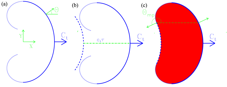
Figure 1. Shape of a wave segment. (a) Segment front (thick solid line) specified by equations (14) and (15) computed for  . The dotted lines represent a continuation of this solution into the region of the segment back. (b) The dashed lines represent the phase wave at the wave back obtained by a shift of the wave front to the left by
  . The thick solid and the dotted lines are the same as in (a). (c) The whole segment boundary with smoothly connected dotted and dashed lines. The thin arrows show the normal directions at the matching point and the corresponding point at the segment front, which was shifted along the dashed–dotted line.
Download figure:
Standard image High-resolution imageOn the other hand, according to the reaction-diffusion equation (1), the normal velocity of a curved wave front should depend on its curvature [4]. For instance, in order to specify this relationship in the case of a concentrically expanding circular wave, the Laplacian in equation (1) can be written in a polar coordinate system that gives

Taking into account that the gradient  is small everywhere except at the thin front region, equation (7) can be simplified further to give

where R is the front curvature radius.
Comparing equation (8) and equation (1) and taking into account equation (4), it becomes clear that the normal velocity in the KL model obeys the linear eikonal equation

where  is specified by equation (5) and
  is the local curvature.
Substituting this eikonal equation into equation (6) and taking into account that  , the description of the segment front can be reduced to a single equation for the angle

To make the consideration more transparent and general, it is useful to use dimensionless velocities and space variables rescaled as  ,
,  ,
,  , and
, and  . After this rescaling, equation (10) reads

Since  and
and  , it is straightforward to use equation (11) to derive equations for the Cartesian coordinates of the front, which gives


Equations (12) and (13) can be solved analytically, and taking into account the conditions X = 0,  and Y = 0,
  , the Cartesian coordinates of the front can be written as [16]

Thus, for a given value of the normalized velocity of the wave segment  equations (14) and (15) specify the shape of the wave segment front. As an example, the segment front obtained for
  ,
,  , and D=1 is shown in figure 1(a).
It is important to stress that the value of v only starts to grow just behind the wave front and still does not exceed τ. Thus, equation (11) also remains valid for the wave back within a region near the phase change point, where  . Hence, one can use equations (14) and (15) to specify the shape of the segment back as shown by dotted lines in figure 1(a). The local curvature of these lines is so large that the normal velocity is negative.
In contrast to TT waves, the back velocity of a TP wave cannot be determined as a function of the curvature or the inhibitor value. However, it is clear that near the symmetry axis the phase wave at the wave back should simply follow the wave front at a fixed distance  . Thus, the shape of the back should be identical to the front shape, but has to be shifted to the left by the space interval
  , as shown by the dashed line in figure 1(b). It is clear from figure 1(b) that this shift cannot be arbitrarily large, since, at least, an intersection between the dotted and the dashed lines should exist. The suitable choice of the space shift value is illustrated in figure 1(c). The space shift is chosen here in such a way that the part of the wave back obeying equations (14) and (15) is smoothly connected to the shifted segment front representing a phase wave at the segment back. Namely, this smoothness condition determines the selected value τ and the wave segment shape corresponding to the given
  value.
This selection condition can be expressed analytically. Indeed, let angle  determine point of the dotted and dashed lines shown in figure 1(b). Then two conditions should be fulfilled for the lines
  and
and  specified by equations (14) and (15), respectively


where  represents the dimensionless spatial shift between the wave segment front and the phase wave at the segment back. Both equations (16) and (17) reflect the fact that in order to fulfill the smoothness condition, the normal direction at the matching point of the segment back has to be turned by π with respect to the corresponding point at the segment front shifted to the left.
The system of four algebraic equations (14)–(17) can be solved, which gives us an expression for the normal angle at the matching point
where

and the selected value of τ
Note that equations (15)–(17) specify a relationship between  and a dimensionless parameter

Moreover, for the given value of the velocity  the half-width W of the segments can be easily determined after a substitution
  into equation (15), which gives

Analytical expressions in equations (18)–(22) allow us to represent the segment velocity  and the half-width W as functions of the parameter B, as shown in figure 2.
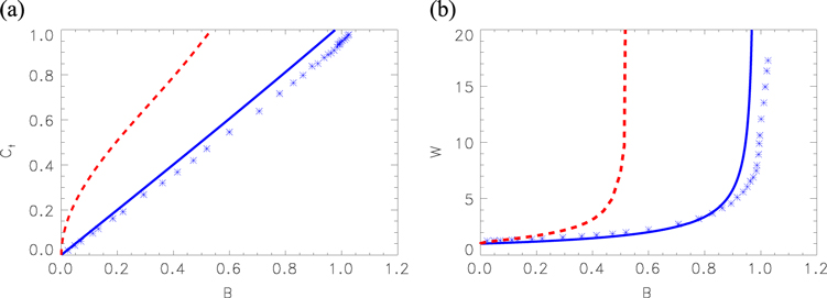
Figure 2. The selected values of the dimensionless segment velocity  (a) and the segment half width W (b) specified by equations (18)–(22) as functions of the dimensionless parameter B (solid lines). The dotted lines show corresponding dependencies found for TT waves in [16]. The results of direct integration of the KL model obtained for D = 1, A = 0.1875,
  , and varying τ are depicted by (*).
Download figure:
Standard image High-resolution imageThese relationships exhibit two limiting cases clearly seen in figure 2. In the first case,  and
and  . The boundary of this practically motionless wave segment approaches a unit circle, and in accordance with equation (14)
  . Substituting this expression into equation (16) and taking into account that
  due to equations (18) and (19), we get the asymptotic

for the segment velocity.
In the second limiting case,  and
and  . The last value can be determined analytically since
  due to equation (19) and
  due to equation (18). Substituting this value into equation (20) gives
  and finally
  . Note that in this limit the segment width diverges, i.e., the wave segment is transformed into a so-called critical finger [14]. In this limiting case, the translational motion of the wave segment of infinitely large width is indistinguishable from a spiral wave rotating at the zero angular velocity.
In the range between these two limits, the relationship  determined by equations (18)–(21) can be approximated as

with accuracy better than 0.1%.
It is important to stress that in the case of TT waves, the translational velocity and the segment width can also be presented as functions of the dimensionless parameter B [16]. At first glance, the definition of the parameter B used in [16] looks quite different with respect to equation (21). However, this definition can be reformulated in terms of the measurable medium parameters [21]. If, in addition, it is taken into account that the parameter τ determines the pulse duration, then both definitions becomes equivalent. The corresponding relationships are shown by dashed lines in figure 2.
Thus, for TP waves as well as for TT waves, the translational velocity of a wave segment and its width are a monotonously increasing function of the same parameter B. However, the obtained relationships look quantitatively differently. First, the critical value  obtained earlier for the critical finger limit is much larger than
  found for TT waves [14–16]. Second, in the limit
  the TP waves obey the linear asymptotic equation (23), while for TT waves the square root relationship
  has been demonstrated [16].
4. Reaction-diffusion simulations
In order to verify the selected relationships, numerous direct numerical integrations of the KL model have been performed. The explicit Euler method has been used with the space step  and the time step
  , and the grid size was
  nodes co-moving with the stabilized wave segment. No-flux boundary conditions have been used.
An example of the numerical data representing the segment velocity and half-width as the functions of the dimensionless parameter B is shown in figure 2. In order to obtain these relationships, the parameters D = 1,  ,
,  , and A = 0.1875 have been fixed in our reaction-diffusion computations, while τ has been varied.
As was mentioned earlier, a translational motion of a wave segment is inherently unstable, but can be stabilized by applying an appropriate feedback to the mediumʼs excitability [6, 7, 15, 22]. In the presented study, a stabilization of the half-width of a propagating wave segment induced in the KL model was achieved by a variation of parameter A in accordance with a linear feedback control

where  and the feedback signal I(t) is specified as

where  is the feedback gain. During the stabilization process, the segment width W(t) oscillates with a decreasing amplitude and finally approaches a stationary value. However, this value is not necessarily equal to the desirable segment half-width
  and, generally speaking, the feedback signal does not vanish. Hence, in accordance with equation (25), the model parameter A will not be equal to a chosen value
  . Therefore, the control scheme based on equations (25) and (26) can be used only if the desirable value of the segment half-width
  is known a priori for a selected value of τ. Since this is usually not the case, in order to achieve a noninvasive stabilization, an additional equation has been included into the control loop

which describes an adaptation of the model parameter τ to the desired value  . The feedback scheme specified by equations (25) through (27) allows us to reach a noninvasive feedback stabilization, i.e., the feedback signal vanishes when the stabilization is completed. Therefore, final W(t) approaches
  and A reaches
  .
.
The results of our simulations obtained commonly with  and
and  are shown in figure 2 and are in quantitative agreement with the predicted values. One reason for the observed deviations, which do not exceed 10%, is the final thickness of the excited domain boundary, which was neglected by the free-boundary approach. Moreover, the whole shape of the stationary propagating wave segments obtained in the reaction-diffusion simulations is in a good agreement with the theoretical predictions obtained in the framework of the free-boundary approach, as shown in figure 3. Of course, in the parameter range
  , where the wave segment width diverges, it makes no sense to compare theoretical and numerical data obtained for the same B. Here, the wave segments propagating at the same velocity
  should be compared. The deviations between the correspondng values of the parameter B do not exceed 10%.
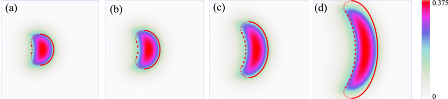
Figure 3. The wave segment obtained from the reaction-diffusion computations (color coded) and by use of the free-boundary approach (solid, dotted, and dashed lines as in figure 1) are presented for (a) B = 0.36, (b) B = 0.52, (c) B = 0.705, and (d) B = 0.86.
Download figure:
Standard image High-resolution image5. Periodic wave train
The results obtained for a single propagating wave can be extrapolated to consider a periodic sequence of wave segments. Note that if the temporal period T of a wave train exceeds  , the value of the variable v along the whole segment front is simply equal to zero. In the opposite case, when
  , the value of v along the whole segment front is equal to T. Substituting v = T into equation (3) specifies the excitation threshold as a function of T.
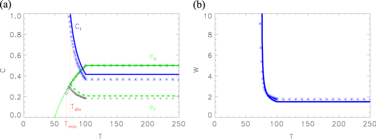
Therefore, the propagation velocity of a planar front determined by equation (4) also depends on T. The dispersion relation  specified by equations (3) and (4) is shown as a thin, solid line in figure 4(a). The results of direct numeric computations of the KL model, depicted by diamonds, indicate that the relationship found analytically is valid practically until
  , the shortest possible period of a one-dimensional wave train. Substituting
  into equation (18) specifies the dimensionless parameter B as a function of T. After this, equations (24) and (22) allow us to obtain
  and
and  , which are shown in figure 4.
Figure 4. The selected values of the dimensionless segment velocity  (a) and the segment half-width W (b) versus the period T of a segment sequence (thick solid lines). Thin solid and dashed lines show the relationships
  and
and  , correspondingly. The results of direct integration of the KL model obtained for
  , A = 0.1875,
  ,
,  , and
, and  are depicted by separate symbols.
Download figure:
Standard image High-resolution image
It can be seen that when T is decreasing, the normalized segment velocity  increases so quickly that the segment velocity
  also increases despite a decrease of
  . At
. At  , the normalized segment velocity reaches
  , i.e.,
  . At this point the segment half-width W diverges and
  , which is the characteristic feature of a critical finger [14]. It is important to stress, that since
  , the dispersion relation determined by equations (3) and (4) is still valid.
6. Summary
In summary, the proposed free-boundary approach allows us to describe analytically the selected values of the propagation velocity and the shape of the stabilized wave segment. These results were extended to consider a periodic segment sequence too. The main result of this consideration is the dimensionless propagation velocity  specified as a monotonously increasing function of a single dimensionless parameter B characterizing the mediumʼs excitability. At B = 0, the segment velocity vanishes and its shape is transformed into a ring of radius
  . For
. For  the velocity
  is simply proportional to B in accordance with equation (20). In contrast to this, a quite different asymptotic
  has been found for TT waves [16].
In the second limiting case, at  , the segment width diverges. This corresponds to the critical finger known for TT waves [14]. However, this transformation occurs at quite different value
  , instead of
  , which was obtained earlier for TT waves [14–16].
More generally, it is demonstrated that the predictions found for TP waves considerably differ from the predictions made for TT waves shown in figure 2. Hence, the results obtained in our study open the possibility to test experimentally what kind of waves can be observed in real excitable systems. It is obvious that the corresponding experiments with wave segments are much easier to perform than those with spiral waves.
Thus, from one point of view, the results obtained in this paper indicate an important role for the dimensionless parameter B as a universal characteristic of the mediumʼs excitability. For TP waves as well as for TT waves, this parameter appears quite naturally after a rescaling of the free-boundary equations that emphasizes its generality. From another side, a strong quantitative difference between the properties of TT and TP waves is clearly demonstrated in the considered example of the stabilized wave segment and earlier in application to spiral waves [12]. A challenge for a future work is to find out other measurable medium parameters that can be used to distinguish TT and TP waves and to characterize in-between situations.