


Abstract
Energy conversion in the machines and information processors of the capital stock drives the growth of modern economies. This is exemplified for Germany, Japan, and the USA during the second half of the 20th century: econometric analyses reveal that the output elasticity, i.e. the economic weight, of energy is much larger than energyʼs share in total factor cost, while for labor just the opposite is true. This is at variance with mainstream economic theory according to which an economy should operate in the neoclassical equilibrium, where output elasticities equal factor cost shares. The standard derivation of the neoclassical equilibrium from the maximization of profit or of time-integrated utility disregards technological constraints. We show that the inclusion of these constraints in our nonlinear-optimization calculus results in equilibrium conditions, where generalized shadow prices destroy the equality of output elasticities and cost shares. Consequently, at the prices of capital, labor, and energy we have known so far, industrial economies have evolved far from the neoclassical equilibrium. This is illustrated by the example of the German industrial sector evolving on the mountain of factor costs before and during the first and the second oil price explosion. It indicates the influence of the 'virtually binding' technological constraints on entrepreneurial decisions, and the existence of 'soft constraints' as well. Implications for employment and future economic growth are discussed.
Export citation and abstract BibTeX RIS

Content from this work may be used under the terms of the Creative Commons Attribution 3.0 licence. Any further distribution of this work must maintain attribution to the author(s) and the title of the work, journal citation and DOI.
1. Introduction: Thermodynamics and economics
On 23 October, 2009 a press release3 appeared, titled: 'The Financial Crisis: How Economists Went Astray. Two Nobel Laureates and over 2000 Signatories Uphold that Economists have mistaken Mathematical Beauty for Economic Truth.' The signatories signed a web petition in support of an article4 by the Nobel Laureate Paul Krugman, saying: 'Few economists saw our current crisis coming, but this predictive failure was the least of the fieldʼs problems. More important was the professionʼs blindness to the very possibility of catastrophic failures in a market economy ... the economics profession went astray because economists, as a group, mistook beauty, clad in impressive-looking mathematics, for truth ...'
This statement reflects a wide-spread feeling among economists that their profession disregards important aspects of real-world economies. It is the purpose of this paper to show that the failure to describe modern economies adequately is not due to the introduction of calculus into economic theory by the so-called 'marginal revolution' during the second half of the 19th century, when the mathematical formalism of physics decisively influenced economic theory. Rather, the culprit is the disregard of the first two laws of thermodynamics and of technological constraints in the theory of production and growth of industrial economies.
A qualitative summary of the first and the second law of thermodynamics says that nothing happens in the world without energy conversion and entropy production. Entropy production density is positive in all irreversible processes, which, of course, include those of economic production. It consists of particle current densities, driven by specific external forces and by gradients of temperature and chemical potentials, and heat current densities, driven by gradients of temperature. A discussion of the environmental impacts of the corresponding emissions, and a rough mathematical modeling of the limits to growth that may result from them, is given in [1]. It concerns problems of the future like climate change. In the present article we constrain ourselves to elucidating the role of energy in the economy by econometric analyses of the past.
Figure 1 shows the model we use for that purpose. This model had been—and is—the intuitive response to the discussions on the limits to growth, which stimulated research on thermodynamcis and economics. It includes energy (more precisely exergy)5 as a third factor of production on an equal footing with the traditional factors capital and labor. In addition, it introduces the factor 'creativity,' which is the specific human contribution to economic growth that cannot be made by any machine capable of learning. Creativity works via ideas, inventions and value decisions and is coupled to the flow of time t. The space available for the evolution of the production system provides natural resources, production sites and absorbs emissions6 . Work performance and information processing by the production factors (instrumental) capital K, labor L, and energy (conversion) E are the basic processes that produce the material wealth represented by the value added of goods and services. These products represent the output Y of the economy. The capital stock K consists of all energy-converting devices and information processors and the buildings and installations necessary for their protection and operation. Value added per year Y and capital K are measured in constant currency by the national accounts, labor L is given in 'hours worked per year' by the national labor statistics, and energy E is measured by the national energy balances in, e.g., 'petajoules converted per year.' Obviously, there is no quantitative ex ante measure of creativity; nevertheless creativityʼs impact can be determined ex post, as it is done in section 3.
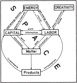
Figure 1. The capital–labor–energy–creativity (KLEC) model of wealth production. Reproduced from [1], chapter 4, p 174, with kind permission of Springer Science + Business Media.
Download figure:
Standard image High-resolution imageEconomic actors decide how much of the factors  , and E are used in order to produce a certain amount of output Y. According to a fundamental behavioral assumption of neoclassical economics the factors are combined in such quantities that the economy operates in an equilibrium that is determined either by the optimization of profit or of time-integrated utility (welfare). We apply these optimization principles to energy-dependent economies in section 2 [1, 3]. In so doing, we take technological constraints on
  and E into account, which have been ignored so far, and disprove the general validity of the fundamental cost-share theorem of standard economics. This theorem says that the economic weight of a production factor, which is called the output elasticity of that factor, should always be equal to the factorʼs share in total factor cost. In highly industrialized countries during the second half of the 20th century, the share of energy in total factor cost has been roughly a meager 5%, while the share of labor has been about 70 and that of capital 25% [4]. Consequently, if energy has been considered at all, only a marginal role has been attributed to it by mainstream economics.
According to the cost-share theorem, reductions of energy inputs by up to 7%, observed during the first energy crisis 1973–1975, could have only caused output reductions of 0.35%, whereas the observed reductions of output in industrial economies were up to an order of magnitude larger. Thus, from this perspective the recessions of the energy crises are hard to understand. In addition, cost-share weighting of production factors has the problem of the Solow residual. The Solow residual accounts for that part of output growth that cannot be explained by the input growth rates weighted by the factor cost shares. It amounts to more than 50% of total growth in many countries. Standard neoclassical economics attributes the discrepancy between empirical and theoretical growth to what is being called 'technological progress' or, sometimes, 'Manna from Heaven.' The dominating role of technological progress 'has lead to a criticism of the neoclassical model: it is a theory of growth that leaves the main factor in economic growth unexplained' [5], as the founder of neoclassical growth theory, Robert A Solow, stated himself.
The observation that since the Industrial Revolution technological progress has manifested itself in increasing numbers of energy-converting devices and information processors, driven by increasing energy inputs and improved by innovations, suggests that 'technological progress' results from the cooperation of the production factor energy with capital, labor, and human creativity, as indicated in figure 1. This is the pre-analytic vision that has guided the research presented in this paper.
Econometric analyses of economic growth in Germany, Japan and the USA during the second half of the 20th century are the subject of section 3. They result in output elasticities that are for energy are much larger and for labor much smaller than the cost shares of these factors. That this is compatible with technologically constrained profit maximization is shown in section 4 by the path of the German industrial sector in its cost mountain. 'Summary and outlook' points out social and ecological problems that arise from the pivotal role of energy in economic growth.
2. Equilibrium from profit and welfare optimization
Mainstream economics is essentially interested in the behavior of economic actors on markets and models it mathematically in formal analogy with classical mechanics. Söllner [6] presents a modern review of this analogy. He points out why and how the 19th-century neoclassical pioneers like Jevons, Edgeworth, and Walras developed the mathematical formalism of economics in a rather close one-to-one correspondence to classical mechanics, especially Newtonian mechanics of the point-like mass; see also [7]. In this formalism, extremum principles of classical mechanics like the minimization of energy, or Hamiltonʼs principle of least action, are the godfathers of the principles of profit or welfare optimization used in economics to determine the equilibrium where an economic system is supposed to operate7 .
In equilibrium, the variables of a system adjust within given constraints in such a way that a system-specific objective becomes an extremum. Let us look into the equilibria that result from profit and welfare optimization.
2.1. Production function and growth equation
A production function  expresses the value added Y of the goods and services produced in an economic system as a function of the production factors and time. The output Y is the gross domestic product (GDP) of a national economy, or a part of the GDP produced by an economic subsector. Y is a state function8
of the inputs
expresses the value added Y of the goods and services produced in an economic system as a function of the production factors and time. The output Y is the gross domestic product (GDP) of a national economy, or a part of the GDP produced by an economic subsector. Y is a state function8
of the inputs  in the same sense as the potential energy of a particle in a conservative force field, or thermodynamic potentials like Gibbʼs free energy, are state functions of their spatial or thermodynamic variables.
The growth equation

which is just the total differential of the production function  , divided by Y, is governed by the output elasticities of capital, α, labor, β, and energy, γ, defined as

 , and γ measure, how the growth rate of output,
  , depends on the growth rates
  ,
,  ,
,  of the inputs
  . From equations (1) and (2) we see that the output elasticity of a production factor measures the productive power of the factor in the sense that (roughly speaking) it gives the percentage of output change when the factor changes by 1%, while the other factors stay constant. Since they give the economic weights (productive powers) of the production factors, the output elasticities are of fundamental importance for the theory of production and growth. δ in equation (1) describes the influence of creativity, with t0 being the base year of the time-series analysis performed in section 3; we will see that creativity manifests itself in time-changing technology paramenters.
At any fixed time t an increase of all inputs by the same factor κ must increase output by κ, because at the fixed state of technology that exists at the given time t a, say, doubling of the production system doubles output; in other words: two identical factories with identical inputs of capital, labor and energy produce twice as much output as one factory. Thus, the production function must be linearly homogeneous in  . As a consequence, the Euler relation, in combination with equation (2), yields the so-called 'constant returns to scale' relation:

2.2. Technological constraints on  , and E

Capital, labor, and energy can be treated as independent variables within a certain region of positive  -space. This region is constrained technologically by the limit to the degree of capacity utilization
  and the limit to the degree of automation
  . As pointed out in [1, 3], we have

The parameters  , λ, and ν can be determined from empirical data on capacity utilization. An example is given in section 4. Km(Y) is the capital stock that would be required for maximally automated production of a given output Y; in this state of the economy, an additional unit of labor would contribute no longer to the growth of output.
Obviously,  cannot exceed unity, because the capital stock cannot work at more than full capacity. (Energy inputs that exceed the power limits the machines are designed for, do not make more productive use of the capital stock. Rather, they may damage the machines; and too much heating or cooling of rooms is also counterproductive. Neither does it make sense to employ more workers than a production system, working at full capacity, requires for its operation and maintenance.) Furthermore, in a given state of technology at time t, the degree of automation of the capital stock has a limit
  at
at  . This limit depends on the mass and the volume of the energy-conversion devices and information processors the production system can accomodate when producing the output Y. The outmost limit to automation is 1, when
  and
and  . Thus, the technological constraints on the combinations of capital, labor, and energy are

The behavioral assumptions that firms maximize profit and individuals maximize welfare originate from microeconomics. But they are also applied to macroeconomic systems [4, 8]. Much more important than the difference between these two assumptions is the difference between neglect and non-neglect of the technological constraints (5) when calculating the equilibria in which macroeconomic systems supposedly operate at a given time t. In order to elaborate that, it is sufficient to look into the necessary conditions for profit and welfare maximization.
For notational convenience we identify  with the components
  of the vector

In this notation, and with the help of the slack variables  and
and  , the constraints (5) can be brought into the form of equations,

The slack variables for labor, energy, and capital are  and
and  . They define the range in factor space within which the factors can vary independently at time t. Inserting them into equation (4) yields the the explicit form of equation (7) as

2.3. Optimization of profit
We assume that the three production factors  have the exogeneously given prices per factor unit
  , so that total factor cost is
  . Economic equilibrium is defined as the state in which profit

is maximum.
The necessary condition for a maximum of profit  , subject to the technological constraints (8), is:
where  is the gradient in factor space;
  and
and  are Lagrange multipliers. (The sufficient condition for profit maximum involves a sum of second-order derivatives. One assumes that the extremum of profit at finite Xi is the maximum.) Equation (10) yields the three equilibrium conditions

Multiplication of (11) with  , and writing the output elasticities
  , defined in equation (2), as

brings the equilibrium conditions into the form
One can write these equilibrium conditions as
by summing the left and right hand sides of (13) over  , observing that
  acording to (3), and expressing Y by the other terms in the resulting relation. The si are

They map the constraints into monetary terms in our nonlinear optimization. We call them 'generalized shadow prices'—'generalized,' in order to avoid confusion with the concept of 'shadow prices,' which refers to terms of the same form one obtains in linear optimization9
. The Lagrange multpliers  and
and  depend on the factor prices pi, the production function Y, and the derivatives of
  . Y cannot be known without knowledge of the output elasticities
  . Equations (14) would only be suited for computing output elasticities, if the neoclassical optimum would lie within the region of
  space that is accessible in the presence of the technological constraints (5). This is not the case for the prices of capital, labor, and energy we have known so far. Figure 6 shows an example how the constraint from capacity utilization prevents an economic system from 'rolling downhill' in its cost mountain—toward the region where profit would be maximum.
But in the absence of technological constraints, all of positive  space would be accessible to the economic system, the Lagrange multipliers
  ,
,  and the generalized shadow prices si would be zero, and the equilibrium conditions (14) would turn into the cost-share theorem: on the rhs of equation (14) the numerator would be the cost
  of the factor Xi, the denominator would be the sum of all factor costs, and the quotient, which is equal to the output elasticity
  , would represent the cost share of Xi in total factor cost.
This would also justify the neoclassical duality of production factors and factor prices, according to which all relevant economic information on production is in the prices. This duality, which is often used in orthodox growth analyses, is a consequence of the Legendre transformation that results from the requirement that profit  is maximum without any constraints on
  . Then equation (11) would hold with
  and yield equilibrium values
  . With
  the profit function would turn into the price function

The essential information on production would be contained in the price function  , which is the Legendre transform of the production function
  . (This is in formal analogy to the Hamilton function being the Legendre transform of the Lagrange function in classical mechanics, or to enthalpy and free energy being Legendre transforms of internal energy in thermodynamics.) However, because of the technological constraints and the resulting generalized shadow prices, the cost-share theorem and equation (16) are not valid in general. For an understanding of the economy, prices are not enough.
2.4. Optimization of time-integrated utility (welfare)
Maximization of overall welfare is an alternative to the derivation of equilibrium conditions from profit maximization. It tests the sensitivity of the equilibrium relations between output elasticities, on the one hand, and factor quantities and prices, on the other hand, to modified behavioral assumptions. The optimization calculus is performed in analogy to the derivation of the Lagrange equations in classical mechanics; for more details see [1].
In welfare optimization one assumes that society maximizes (undiscounted) time-integrated utility U [8]. The integral W is called (overall) welfare. We take it between the times t0 and t1, during which the relevant variables evolve along a curve symbolized by ![$[s]$](https://content.cld.iop.org/journals/1367-2630/16/12/125008/revision1/njp505353ieqn63.gif) . We limit the calculation to the simplest case that the utility function U only depends on consumption C:
. We limit the calculation to the simplest case that the utility function U only depends on consumption C: ![$U=U[C]$](https://content.cld.iop.org/journals/1367-2630/16/12/125008/revision1/njp505353ieqn64.gif) . A simple function with the property of decreasing marginal utility10
is, for instance,
. A simple function with the property of decreasing marginal utility10
is, for instance,

Macroeconomic consumption is the difference between output and capital formation.
Thus, the optimization problem is: maximize overall welfare

subject to the technological constraints (8) and the additional economic constraint that the total cost  of producing consumption C by means of the factors
  must not diverge. Rather, its magnitude cf (t) must be finite at all times t, where each price per factor unit, pi, is exogeneously given:

Therefore, besides  and
and  , the variational formalism of intertemporal welfare optimization includes the Lagrange multiplier μ, which takes care of (19). The curve
 ![$[s]$](https://content.cld.iop.org/journals/1367-2630/16/12/125008/revision1/njp505353ieqn69.gif) , of which
, of which ![$W[s]$](https://content.cld.iop.org/journals/1367-2630/16/12/125008/revision1/njp505353ieqn70.gif) is a functional, depends on the variables that enter consumption C. Output (per unit time) is described by the macroeconomic production function
is a functional, depends on the variables that enter consumption C. Output (per unit time) is described by the macroeconomic production function  . Part of Y goes into consumption C and the rest into new capital formation
  plus replacement of depreciated capital. Economic research institutions provide the price of capital utilization p1 as the sum of net interest, depreciation and state influences. We use this price. Since it already includes depreciation, we can omit explicit reference to the depreciation rate, so that consumption is given by

All taken together we have to optimize

Thus, ![$W[s]$](https://content.cld.iop.org/journals/1367-2630/16/12/125008/revision1/njp505353ieqn73.gif) is a functional of the curve
is a functional of the curve ![$[s]=\{t,{\bf X}:\quad {\bf X}={\bf X}(t),\ {{t}_{0}}\leqslant t\leqslant {{t}_{1}}\}$](https://content.cld.iop.org/journals/1367-2630/16/12/125008/revision1/njp505353ieqn74.gif) .
.
Consider another curve ![$[s,{\bf h}]=\{t,{\bf X}:\quad {\bf X}={\bf X}(t)+{\bf h}(t),\ {{t}_{0}}\leqslant t\leqslant {{t}_{1}}\}$](https://content.cld.iop.org/journals/1367-2630/16/12/125008/revision1/njp505353ieqn75.gif) close to
close to ![$[s]$](https://content.cld.iop.org/journals/1367-2630/16/12/125008/revision1/njp505353ieqn76.gif) , which goes through the same end points so that
, which goes through the same end points so that  . Its functional
 ![$W[s,{\bf h}]$](https://content.cld.iop.org/journals/1367-2630/16/12/125008/revision1/njp505353ieqn78.gif) is obtained from
is obtained from ![$W[s]$](https://content.cld.iop.org/journals/1367-2630/16/12/125008/revision1/njp505353ieqn79.gif) by changing
by changing  to
to  and
and  to
to  everywhere in the integrand of equation (21). Since
  is small, the integrand can be approximated by its Taylor expansion up to first order in
  and
and  .
.
The necessary condition for the maximum of overall welfare is that the variation ![$\delta W\equiv W[s,{\bf h}]-W[s]$](https://content.cld.iop.org/journals/1367-2630/16/12/125008/revision1/njp505353ieqn87.gif) vanishes.
vanishes.  contains the time integral of
Partial integration shifts the time derivative from  to the functions multiplying it. Then, the integrand in
  is a sum of terms that multiply
  . The condition

is satisfied, if these terms vanish. Observing (20) one sees that they do, if

the Kronecker delta  , is 1 for i = 1 and 0 otherwise11
.
, is 1 for i = 1 and 0 otherwise11
.
Equations (24) are the general equilibrium conditions for an economic system subject to cost limits and technological constraints, if the behavioral assumption is that society optimizes time-integrated utility. They correspond to the equilibrium conditions (11) from profit optimization. The difference between the two equilibrium conditions becomes negligible under the conditions indicated below equation (25).
Dividing equations (24) by  and multiplying them by
  produces the output elasticities
  on the lhs, and the rhs involves terms that, after some manipulations, can be brought into the form of (modified) generalized shadow prices

With these modified si the equilibrium conditions (24) assume the form of equation (14).
The shadow prices (25) differ from those of (15) in two aspects. First, there is the term  . This term originates from equation (20) and is due to taking capital formation into account in intertemporal utility optimization, whereas capital formation is no issue in profit optimization. It vanishes, if one can disregard decreasing marginal utility and approximate the utility function
 ![$U[C]$](https://content.cld.iop.org/journals/1367-2630/16/12/125008/revision1/njp505353ieqn99.gif) in (17) by its Taylor expansion up to first order in
in (17) by its Taylor expansion up to first order in  . Second, the ratios
  ,
,  of Lagrange multipliers take the positions of the Lagrange multipliers
  ,
,  in (15). If one does profit maximization subject to the additional constraint
  , which fixes factor cost, one gets the quotients of the Lagrange multipliers as in (25). Thus, the second difference is rather a formal one.
As in profit maximization, because of the technological constraints the cost-share theorem is not generally valid in intertemporal utility maximization.
2.5. Virtually binding and soft constraints
From here on we consider economies that cannot operate in the neoclassical maximum of profit or welfare, because the barriers from the technological constraints and the associated generalized shadow prizes block the access to this maximum. Consequently, the equilibrium point may be either in the interior or at the boundary of the accessible region in  space.
Suppose an economy has the maximum of its objective function right at a barrier, where the '=' sign holds in (5). Nevertheless, it might not operate there either, because of several reasons not taken into account so far. For instance, entrepreneurs prefer combinations of  , in which the quantities of labor L and energy E, which handle and power the capital stock K of a certain degree of automation ρ, produce an output
  that meets demand. Since demand is fluctuating, entrepreneurs have to adjust the degree of capacity utilization η, defined in (4), accordingly. This cost-saving flexibility requires operation in points of factor space that are positioned at some distance from the barrier at
  . In such a situation, the technological constraint on the degree of capacity utilization acts as a 'virtually binding' constraint.
Conceivably, there are yet other aspects that keep the economy at some distance from the constraint barrier(s). For instance, entrepreneurs may not wish to automate the capital stock as much as the technological limit  would allow, because they would have to pay compensations to laid-off workers according to contracts and negotiations with labor unions; legal and social obligations may matter as well. We call these aspects 'soft' constraints.
Thus, realistic economic decision makers operate in regions of  space, where the '<' sign holds in equations (5) and where
  , and E are independent variables.
3. Energy and economic growth
An alternative method that is needed for computing output elasticities has been developed in studies on energy and economic growth, which are reviewed in [1]. It is sketched subsequently, and its main results are presented.
3.1. Computing output elasticities and production functions
Production functions  , which describe economic evolution, are state functions and integrals of the growth equation (1) along a convenient path in factor space from an initial point
  with Y0 at time t0 to the point
  at the time of interest t. It is convenient to work with quantities that are normalized to their magnitudes in the base year t0. Thus, we work with the dimensionless variables

The growth equation (1) and the output elasticities (2) are invariant under the transformations (26).
The production function ![$y[k,l,e;t]$](https://content.cld.iop.org/journals/1367-2630/16/12/125008/revision1/njp505353ieqn116.gif) as a state function of
as a state function of  must be twice differentiable with respect to
  . This results in the partial differential equations

for the output elasticities, where (3) has been taken into account. These equations correspond to the Maxwell relations in thermodynamics. The most general solutions of (27) are

here  and
and  are any differentiable functions of their arguments. The output elasticities, and thus the combinations of
  , must satisfy the restrictions

which result from the technical-economic requirement that all output elasticities must be non-negative. Otherwise, the increase of an input would result in a decrease of output—a situation the economic actors will avoid.
It is not hard to verify with the help of equations (1) and (28) that the corresponding general form of the twice-differentiable, linearly homogeneous production function is given by the rhs of

where  .
.
We insert (30) into the growth equation that results from (1) by the transformation (26) to dimensionless variables. This yields

The economic boundary conditions that would allow to determine the output elasticities (28) and the production function (30) exactly for a given economic system are not known, and never will be, because—according to the theory of partial differential equations—they would require knowledge of β on a surface and of α on a curve in  space. In this sense, all output elasticities and production functions are approximations.
The simplest solutions of equation (27) are constant output elasticities  ,
,  , and
, and  . The corresponding integral of the growth equation is the energy-dependent version of the well-known Cobb–Douglas production function:

The simplest factor-dependent solutions are the output elasticities  ,
,  , and
, and  . With these elasticities integration of the growth equation yields the (first) LinEx production function,

which depends linearly on energy and exponentially on factor quotients. Here  , and
, and  are technology parameters: a indicates capital efficiency, and c indicates the energy demand of the fully utilized capital stock. Innovations may change them in time and contribute to δ in equation (1). The output elasticity of capital,
  , vanishes for vanishing ratios of labor and energy to capital and thus reflects the law of diminishing returns. The output elasticity of labor,
  vanishes, when the capital stock approaches the magnitude km required for maximum automation, and when simultaneously the energy input approaches the quantity em = ckm that is demanded by the fully utilized capital stock km.
The technology parameters  and y0 of the LinEx function are determined from the empirical time series of output yempirical(t). We allow for time dependencies of the technology parameters and model them by logistic functions [10], which are typical for growth in complex systems and innovation diffusion. Alternatively, we have used Taylor expansions of a(t) and c(t) in
  . The free coefficients of the logistics, or of the Taylor expansions, are determined by minimizing the sum of squared errors

The sum goes over all years ti between the initial and the final observation time. It contains the empirical time series of output  , and the LinEx function
  with the empirical time series of k, l and e as inputs at times ti. Minimization is subject to the restrictions (29). Methodological details and the empirical time series of
  are given in [1].
3.2. Growth in Germany, Japan, and the USA
The reproduction of economic growth in Germany, Japan, and the USA during the second half of the 20th century by the LinEx function is shown in figures 2–5. These figures are taken from [11]. Their left parts exhibit the empirical growth (squares) and the theoretical growth (circles) of the dimensionless output  , and the right parts present the empirical time series of the dimensionless factors capital
  , labor
  , and energy
  . The base year t0 is 1960 for Germany and the USA, and 1965 for Japan. Note the variations of inputs and outputs in conjunction with the oil price explosions. The price of a barrel of crude oil in inflation-corrected
  was driven by the OPEC boycott in response to the Yom-Kippur war from 15$ in 1973 to 53$ in 1975, and by the war between Iraque and Iran from 48$ in 1979 to 100$ in 1981. Then the oil price plummeted to 30$ in 1986 (with dramatic consequences for the Soviet Union). Between 1997 and 2011 it has risen again, from 18$ to 110$.
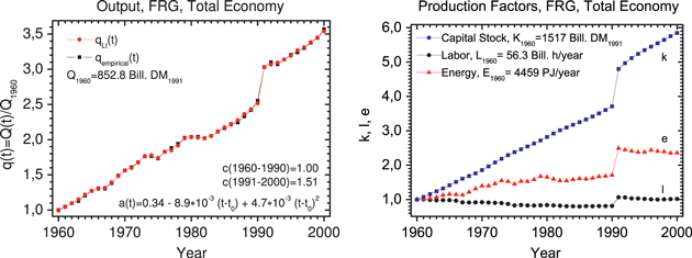
Figure 2. Growth in the total economy of the Federal Republic of Germany (FRG) between the years 1960 and 2000. The five coefficients, shown below the output graph, model the time dependence of the LinEx–function parameters a and c. They reproduce the drastic structural break at German reunification in 1990. Reproduced from [1], chapter 4, pp 206–208, with kind permission of Springer Science + Business Media.
Download figure:
Standard image High-resolution imageThe time-averaged output elasticities of capital,  , labor,
  , energy,
  , and creativity,
  , are presented in table 1 for the economic systems: FRG TE (total economy of the Federal Republic of Germany before and after reunification), FRG I (German industrial sector 'Warenproduzierendes Gewerbe' (GWG)), Japan I (Japanese sector 'Industries'), and USA TE (total economy of the USA). R2 is the adjusted coefficient of determination, and dW is the Durbin–Watson coefficient (whose best value is 2). Both statistical quality measures are quite good.
Table 1. Time-averaged LinEx output elasticities and statistical quality measures. Reproduced from [1], chapter 4, pp 206–208, with kind permission of Springer Science + Business Media.
| FRG TE | FRG I | Japan I | USA TE | |
|---|---|---|---|---|
| System | 1960–2000 | 1960–99 | 1965–92 | 1960–96 |

|
0.38 ± 0.09 | 0.37 ± 0.09 | 0.18 ± 0.07 | 0.51 ± 0.15 |

|
0.15 ± 0.05 | 0.11 ± 0.07 | 0.09 ± 0.09 | 0.14 ± 0.14 |

|
0.47 ± 0.1 | 0.52 ± 0.09 | 0.73 ± 0.16 | 0.35 ± 0.11 |

|
0.19 ± 0.2 | 0.12 ± 0.13 | 0.14 ± 0.19 | 0.10 ± 0.17 |
| R2 | >0.999 | 0.996 | 0.999 | 0.999 |
| dW | 1.64 | 1.9 | 1.71 | 1.46 |
We note that for all the systems considered the output elasticity of energy is much larger than energyʼs cost share of roughly 5%, and the output elasticity of labor is much smaller than laborʼs cost share of about 70%. The economic weight  of creativity, computed from the time changes of a(t) and c(t), is comparable to that of labor,
  .
.
Ayres and Warr have analyzed economic growth in the USA during the 20th century, using 'useful work' as the energy variable in the LinEx function. 'Useful work' is defined as exergy, multiplied by appropriate conversion efficiencies, plus physical work by animals. The 'useful work' data [12] already include most of the efficiency improvements that have occurred in the energy converting systems of the USA during the 20th century. In this case two constant technology parameters suffice to reproduce well the gross domestic product of the US economy between 1900 and 1998 [13, 14]. The time averages of the corresponding output elasticities of capital, labor and 'useful work' are similar to the ones in table 1.
These findings are supported by cointegration analyses [15]. The energy-dependent Cobb–Douglas function (32), whose constant output elasticities are similar to the time-averaged LinEx output elasticities, also reproduces economic growth more or less satisfactorily, albeit with larger discrepancies between theoretical and empirical growth during and after the 1973–1981 oil-price shocks [1, 14].
The reproduction of economic growth in Germany, Japan, and the USA during up to four decades with small residuals, and output elasticities that are for energy much larger and for labor much smaller than the cost shares of these factors, are the principal results of the KLEC-model applied in this section. The contribution of human creativity to growth appears as comparable to that of labor12
. The fundamental presumption of the model is, that the macroeconomic production function  (and its dimensionless version
  as well) is a state function of the economic system, so that its infinitesimal change is a total differential and the integral of this differential between
  and
and  does not depend on the path in factor space. Such
  must be twice differentiable with respect to
  . From this property follow the growth equation (1) and the partial differential equations (27) for the output elasticities13
. Essential is that the output elasticities are not set equal to the cost shares, as it is done in mainstream economics, but that instead they are determined by fitting the production functions to the time series of output, where the restrictions (29)—output elasticities must be non-negative—have to be observed.
. From this property follow the growth equation (1) and the partial differential equations (27) for the output elasticities13
. Essential is that the output elasticities are not set equal to the cost shares, as it is done in mainstream economics, but that instead they are determined by fitting the production functions to the time series of output, where the restrictions (29)—output elasticities must be non-negative—have to be observed.
A number of analyses of past growth with alternative energy-dependent production functions, whose output elasticities satisfy (27), have yielded results similar to the ones presented here [1, 7]. Cobb–Douglas functions are the work-horses of mainstream econometrics. Unfortunately, they ignore the physical restrictions on factor substitution. But since the economic actors are aware of these restrictions, Cobb–Douglas is not too bad for reproductions of past economic growth, despite the insensitivity of the constant output elasticities to input fluctuations. (For scenarios of the future, however, the law of diminishing returns and the approach to the state of maximum automation should be incorporated in the output elasticities, as it is exemplified by the LinEx function (33).) The choice of the base year and the methods to minimize the sum of squared errors SSE (34) have had little influence on the econometric findings so far14 . Energy-dependent service production functions also reproduce the growth of the (West) German service sector quite well, yielding output elasticities of energy and labor that deviate from these factors' cost shares not quite as much as in the total economy [7, 16]. The increasing automation in agriculture and industries shifts more and more of the labor force into the less energy-intensive service sector. Nevertheless, computer- and electricity-based automation is progressing in that sector, too, especially in finance, logistics, and retail business.
Whatever the details of modeling energyʼs working as a factor of production, one result is common to all models:
If one foregoes cost-share weighting and determines the output elasticities of capital, labor, energy, and creativity econometrically, one gets for energy economic weights that exceed energyʼs cost share by up to an order of magnitude, and the Solow residual disappears. The production factor energy accounts for most, and creativity for the rest of the growth that neoclassical economics attributes to 'technological progress'.
4. Economic evolution in the cost mountain
We consider the mountain of factor cost that rises above the plane that is spanned by the input ratios 'labor/capital' ( ) and 'energy/capital' (
 ). The cost PY of producing a given output
 ![$Y(t)=Y[K,L,E;t]$](https://content.cld.iop.org/journals/1367-2630/16/12/125008/revision1/njp505353ieqn167.gif) is obtained by multiplying the time-dependent prices per capital unit, pK(t), labor unit, pL(t), and energy unit, pE(t), by the factor quantities
is obtained by multiplying the time-dependent prices per capital unit, pK(t), labor unit, pL(t), and energy unit, pE(t), by the factor quantities  required to produce that output:
  , where
  .
.
In order to relate the total factor cost at time t to the output at t we rewrite ![${{P}_{Y}}=e[{{P}_{K}}k/e+{{P}_{L}}l/e+{{P}_{E}}]=e[{{P}_{K}}/v+{{P}_{L}}u/v+{{P}_{E}}]$](https://content.cld.iop.org/journals/1367-2630/16/12/125008/revision1/njp505353ieqn171.gif) , remember that
, remember that  on the lhs of equation (30), rewrite this equation in the form
  , insert this into the equation for PY, and obtain the equation of the cost mountain as

The cost mountain rises above the  plane, its topography is determined by the prices and ratios of the production factors, and its height scales with
  .
.
The profit GY obtained from the output Y is  . Profit maximum means that

is minimum. Since the cost mountain and the mountain of negative profit just differ by the height-shift Y(t), the structure of both mountains is the same.
The negative gradient,  , of
, of  points in the direction where the economy would move, if the economic actors would only have the objective of profit maximization;
  and
and  are the unit vectors parallel to the u-axis and the v-axis that span the
  plane. Operating with
  on
on  in equation (36), and observing that equation (31) leads to
  and
and  , one obtains the gradient of profit

as the negative gradient of the cost mountain with the components


To visualize the trajectory of a real-life economy on the slope of its cost mountain, the time-changing factor prices, the inputs, and an appropriate production function  are needed in equations (35), (38), and (39). The production function should reproduce economic growth reasonably well with small residuals and acceptable statistical quality measures. As we have seen in section 3, the LinEx function (33) satisfies these criteria. The energy-dependent Cobb–Douglas function (32) with output elasticities that are close to the time-averaged LinEx output elasticities in table 1 may also be considered as an acceptable production function until the second oil-price shock.
In figure 6 the trajectory of the GWG in the cost mountain and the negative cost gradients are projected onto the mountain base, as an example. We use this example, because the sector GWG is the pillar of the German economy—it produced about 50% of (West) German GDP in the 1960s and 1970s—,and its aggregated, inflation-corrected energy prices are available from a research project carried out in the 1980s [17]. At the time of this project, factor prices could only be constructed for the times between 1960 and 1981. The directions of the negative cost gradients in figure 6 are relatively little affected by the two oil-price explosions, because the latter varied energyʼs small cost share only between 4% and 7%. Neither has this direction changed much between 1981 and 1989. The structural break in the German economy at reunification in 1990, which shows in the growth curves of GWG in figure 3, would make it rather difficult to construct a consistent set of updated, inflation-corrected, aggregated energy price data since then. Therefore, we constrain ourselves to the time between 1960 and 1989 in this illustrating example.
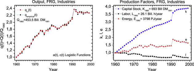
Figure 3. Growth in the German industrial sector 'Warenproduzierendes Gewerbe' (GWG) between 1960 and 1999. Reproduced from [1], chapter 4, pp 206–208, with kind permission of Springer Science + Business Media.
Download figure:
Standard image High-resolution imageDuring the first and the second oil-price shock the aggregate energy price increased in Germany by a factor of 2.5. Similar price shocks hit the other industrial market economies and triggered their first two serious post-war recessions. During these recessions, the variations of economic output closely followed the variations of energy input, as figures 2–5 show. Since then, energy conservation measures have been taken, and energy-intensive, polluting production processes have been shifted abroad. As a result, the technology parameters a and c of the LinEx function acquire a time dependence, which, however, has been negligible for the time span covered by the trajectory in figure 6.
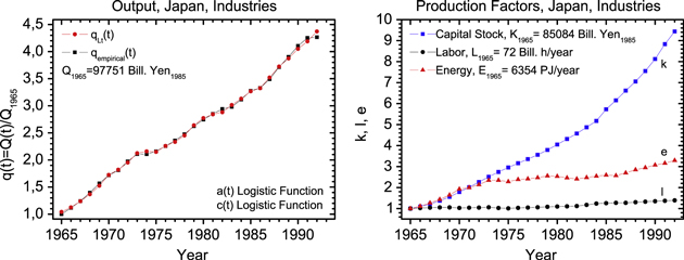
Figure 4. Growth in the Japanese sector 'Industries,' which produces about 90% of Japanese GDP, between 1965 and 1992. Reproduced from [1], chapter 4, pp 206–208, with kind permission of Springer Science + Business Media.
Download figure:
Standard image High-resolution image
Figure 5. Growth in the total US economy between 1960 and 1996. Reproduced from [1], chapter 4, pp 206–208, with kind permission of Springer Science + Business Media.
Download figure:
Standard image High-resolution imageThe barrier from the constraint that capacity utilization cannot exceed 1, see equations (5) and (7), is written in terms of the dimensionless inputs as

where the parameters λ, ν, and  have been determined by fitting the rhs of equation (40) to empirical data on capacity utilization in the German economy. These data, published by the 'Sachverständigenrat für die Gesamtwirtschaft,' are given in [7]. The parameters
  reproduce the data satisfactorily, although the fit stays somewhat below the maxima in 1965, 1969, and 1970. The barrier from the technological constraint (40) is indicated by the full squares in figure 6. The LinEx function indicates that the barrier from maximum automation is in the region where
  , so that
  , and where
  .
.
Direction and length of the arrows above the trajectory indicate directions and strengths of the negative cost gradients, whose components are calculated with the LinEx production function; arrow lengths are for the 1970 output quantity. Below the path, the lines without arrow heads indicate the negative cost gradients obtained with an energy-dependent Cobb–Douglas function whose output elasticities are close to the time-averaged elasticities of the LinEx function. The gradients depend little on the type of production function. What matters is the magnitude of the output elasticities. The general direction of the trajectory is at a large angle to the negative cost gradients, which point toward the region of small  and much larger
  . Only during times of economic upswings, as from 1967–1970, 1972–1973, and 1975–1979, the path follows the negative cost gradients toward the barrier from the limit to capacity utilization temporarily. This shows that increasing the energy input into the machines that were not fully employed in times of recessions, rapidly increases output and profit15
. The isolated point for 1989 indicates that, until German reunification in 1990, the general direction of the path toward strongly decreasing u and moderately decreasing v continues. It is more or less parallel to the barrier from the limit to capacity utilization, save for the substantial shift of the empirical trajectory toward the barrier in the late 1960s. Obviously, the virtually binding constraint associated with the limit to capacity utilization and soft constraints, which are discussed in section 2, keep the economic system on the uphill side of the barrier. Along the trajectory in the cost mountain, the inputs of expensive labor are reduced and cheaper energy/capital combinations are substituted for them.
. Only during times of economic upswings, as from 1967–1970, 1972–1973, and 1975–1979, the path follows the negative cost gradients toward the barrier from the limit to capacity utilization temporarily. This shows that increasing the energy input into the machines that were not fully employed in times of recessions, rapidly increases output and profit15
. The isolated point for 1989 indicates that, until German reunification in 1990, the general direction of the path toward strongly decreasing u and moderately decreasing v continues. It is more or less parallel to the barrier from the limit to capacity utilization, save for the substantial shift of the empirical trajectory toward the barrier in the late 1960s. Obviously, the virtually binding constraint associated with the limit to capacity utilization and soft constraints, which are discussed in section 2, keep the economic system on the uphill side of the barrier. Along the trajectory in the cost mountain, the inputs of expensive labor are reduced and cheaper energy/capital combinations are substituted for them.
The Japanese and US empirical data on capital, labor, and energy in figures 4 and 5 show that until 1973 factor growth in the USA and Japan differs from that of Germany: labor grows in the USA, but more slowly than capital, and remains nearly constant in Japan, whereas capital and energy increase at nearly the same rate in both countries. In Germany, on the other hand, labor always decreases16
, and the input of energy grows much less than the capital stock. But after the first oil price shock, the growth of energy is significantly reduced in all three systems, while the growth of capital continues as before. In the USA and Germany the energy input oscillates in response to the oil price variations, and in Japan it nearly flattens out. Consequently, the US and Japanese path in the  plane stays close to a line of constant
  and decreasing
  until 1973, and thereafter both
  and
and  decrease. Then, the economic actors in the USA and Japan seem to behave similar to the ones in Germany.
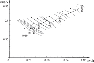
Figure 6. The solid line indicates the path of the German industrial sector 'Warenproduzierendes Gewerbe' (GWG) in the cost mountain between the years 1960 and 1981, projected onto the  plane;
  and
and  , where
  , and e are multiples of capital, labor, and energy in the base year
  . The full squares mark the barrier from the limit to capacity utilization. The way of computing them from equation (40) is described below that equation. They complement (the modified) figure 4 of [17].
Download figure:
Standard image High-resolution image5. Summary and outlook
Energy-dependent production functions, with output elasticities that are for energy much larger and for labor much smaller than the cost shares of these factors, reproduce economic growth in Germany, Japan, and the USA with small residuals and good statistical quality measures—even during the downturns and upswings in the wake of the first and the second oil-price explosion. This does not contradict the usual behavioral assumptions that entrepreneurs maximize profit or that society maximizes overall welfare, because real-world economic actors are aware of the technological and the related 'virtually binding' constraints on the combinations of capital, labor, and energy. 'Soft' constraints from legal and social obligations may also matter. The barriers from the constraints on capacity utilization and automation prevent modern industrial economies from reaching the neoclassical optimum of mainstream economics, where output elasticities would be equal to factor cost shares.
Since in industrially advanced countries cheap energy is economically much more powerful than expensive labor, there has been the long-time trend toward increasing automation, which replaces expensive labor by cheap energy-capital combinations. In the G7 countries, this trend has drastically reduced the number of people employed in the sectors agriculture and industries during the last four decades, and the contribution of these sectors to GDP as well (see, e.g., tables 4.1 and 4.2 in [1]). Now, in the service sector, electricity-powered computers with appropriate software kill more and more jobs, too. The resulting danger of unemployment in the less qualified part of the labor force is enhanced by the trend toward globalization, where goods and services produced in low-wage countries can be delivered at small cost to high-wage countries thanks to cheap energy and increasingly sophisticated, highly computerized transportation systems.
The nearly unanimous social and political response to this danger is the call for strategies to stimulate economic growth. But these strategies face obstacles from entropy production, which is coupled to energy conversion and its pivotal role in economic growth: (1) there are thermodynamic limits to the improvement of energy efficiency at unchanged energy services, because entropy production destroys exergy; (2) emissions associated with entropy production, especially the ones of carbon dioxide from the combustion of fossil fuels, threaten climate stability. The question is, whether society will be willing and able to finance the huge investments that are necessary for the transition to a highly efficient production system powered by non-fossil fuels.
Finally, discussing the possibly decreasing recovery of cheap conventional oil according to the 'peak-oil' theory [18], the International Monetary Fund [19] quotes the high output elasticities of energy reported in [1, 10] and [13] and concludes: '... if the contribution of oil to output proved to be much larger than its cost share, the effects could be dramatic, suggesting a need for urgent policy action.' Further research concerning the impact of energy conversion and entropy production on economic evolution is needed to guide that action.
Footnotes
- 3
From Professor Geoffrey M Hodgson, The Business School, University of Hertfordshire, Hatfield, Hertfordshire AL10 9AB, UK; www.geoffrey-hodgson.info
- 4
New York Times, 2nd September, 2009.
- 5
Energy consists of useful exergy and useless anergy. Exergy can be converted into any form of useful work, whereas anergy is heat dumped into the environment, for instance. Entropy production enhances anergy at the expense of exergy. Since all primary energy carriers taken into account in our analyses (coal, oil, gas, renewables, and nuclear fuels) are basically 100% exergy, we do not discriminate between energy and exergy, where 'energy consumption' means 'exergy consumption.'
- 6
'Space' expands the traditional factor 'land' into the third dimension.
- 7
Ironically, neoclassical economics uses Hamiltonians as in classical mechanics, but these Hamilton functions have nothing to do with energy, which standard economics disregards as a factor of production.
- 8
Substantial critique of factor aggregation and of the neoclassical concept of macroeconomic production functions is discussed in appendix 3 to chapter 4 of [1]. Since work performance and information processing are the primary technical aggregation principles for output and factors, on which we base production functions (where equivalence factors relate technical quantities to monetary ones) [1, 2, 10], our conceptual foundation differs from the criticized one of neoclassical economics.
- 9
The concept of 'generalized shadow prices' is introduced here, because, in general, constrained nonlinear optimization may result in an optimum that is situated in the interior of the accessible region, whereas in linear optimization the optimum always lies on a vertex of the boundary, where constraints are binding. If a nonlinear objective function has a number of extrema in its domain, it may also have an extremum in the interior of the restricted domain that remains accessible when constraints are applied. The 'generalized shadow prices' are calculated by using the
magnitudes for the optimum within the restricted domain; for details see [1, 3]. Contrary to the 'shadow price' from linear optimization, a 'generalized shadow price' is not neccessarily associated with a binding constraint. Gauvin [9] discusses shadow prices in nonconvex programming, using a nonlinear program with equality and inequality constraints. - 10
The utility of consuming an additional piece of bread is less for a satiated person than for a hungry one.
- 11
If one identifies
with the Lagrangian , one sees the formal equivalence of (24) with constrained Lagrange equations of motion in classical mechanics. - 12
Error propagation produces the large errors in
. - 13
- 14
Nevertheless, the Levenberg–Marquardt method in combination with the self-consistent iteration scheme (see appendix 6 of chapter 4 of [1]) for SSE minimization, which is used in [11] to produce the results of this paper, has been so far the one that yields the best statistical quality measures. Furthermore, the LinEx function
in (33) is the simplest one in the family of LinEx functions, some of whose members are presented in [7]. For the energy-dependent Cobb–Douglas function (32) a shift of the base year results in a transformation of the parameter y0CDE, and for the somewhat more complicated LinEx function a base-year shift results in three equations between the parameters , and c of the two sets that belong to the two , whose variables are normalized to their values in the two different base years. For the simple yL1, on the other hand, we know (only) from fitting by SSE minimization, that base-year shifts have negligible influence on the results. - 15
Since the machines of the capital stock are activated by energy, economic causality between output and energy input is bidirectional (at least in the short run, when improvements of energy efficiency have not yet been developed): fluctuations of demand lead to corresponding fluctuations of demand-adjusted production and energy inputs. Fluctuations of energy inputs in the case that an important energy source would dry up and another one would be discovered and opened up, would lead to corresponding fluctuations of output.
- 16
This causes the 'condensation' of the trajectory points with decreasing u in figure 6.

![$U[C({\bf X},{{\dot{X}}_{1}})]$](https://content.cld.iop.org/journals/1367-2630/16/12/125008/revision1/njp505353ieqn93.gif)


![${{y}_{L11}}=y_{L11}^{0}e{\rm exp} \left[ a\left( 1-\frac{l}{k} \right)+\frac{1}{c}\left( 1-\frac{e}{k} \right)+ac\left( \frac{l}{e}-1 \right) \right]$](https://content.cld.iop.org/journals/1367-2630/16/12/125008/revision1/njp505353ieqn162.gif)

