


Abstract
We introduce a new method to measure Lagrangian vorticity and the rotational dynamics of anisotropic particles in a turbulent fluid flow. We use 3D printing technology to fabricate crosses (two perpendicular rods) and jacks (three mutually perpendicular rods). Time-resolved measurements of their orientation and solid-body rotation rate are obtained from four video images of their motion in a turbulent flow between oscillating grids with  = 91. The advected particles have a largest dimension of 6 times the Kolmogorov length, making them a good approximation to anisotropic tracer particles. Crosses rotate like disks and jacks rotate like spheres, so these measurements, combined with previous measurements of tracer rods, allow experimental study of axisymmetric ellipsoids across the full range of aspect ratios. The measured mean square tumbling rate,
  , confirms previous direct numerical simulations that indicate that disks tumble much more rapidly than rods. Measurements of the alignment of a unit vector defining the orientation of crosses with the direction of their solid-body rotation rate vector provide the first direct observation of the alignment of anisotropic particles by the velocity gradients in a turbulent flow.
Export citation and abstract BibTeX RIS

Content from this work may be used under the terms of the Creative Commons Attribution 3.0 licence. Any further distribution of this work must maintain attribution to the author(s) and the title of the work, journal citation and DOI.
1. Introduction
The motion of particulate matter in fluid flows has long been a central problem in both fundamental and applied fluid mechanics. The dynamics of spherical particles was a natural starting point for Stokes, who considered this problem in the 19th century [1]. A long list of researchers continued work to describe the motion of spherical particles at low Reynolds number, leading to the Maxey–Riley–Gatignol equation [2, 3]. The development of numerical simulations [4, 5] and experimental tools [6–8] capable of revealing the motion of spherical particles in complex flows has led to a recent resurgence of work on particle dynamics [9].
Extending the problem to non-spherical particles in general is important for many applications ranging from icy clouds [10], to bio-locomotion [11], to suspension flows in industrial settings [12], among others (e.g., [13, 14]). In 1922, Jeffery analyzed the motion of ellipsoidal particles in Stokes flow [15]. For the case of axisymmetric particles, their tumbling rate can be expressed as

where  is a unit vector along the symmetry axis of the ellipsoid, α is the aspect ratio defined as the ratio of length to diameter,
  is the anti-symmetric part of the velocity gradient tensor (vorticity), and
  is the symmetric part of the velocity gradient tensor (strain rate). Equation (1) is valid for axisymmetric particles, but it has also been extended to tri-axial ellipsoids (see, e.g., [16]). A wide range of studies has explored deviations from Jeffery dynamics due to particle inertia, particle shape, and Reynolds number, among other factors [17]. Analytic work [18, 19] and numerical simulations [20–23] have made significant progress extending studies of non-spherical particles in complex flows, but experimental measurements of the dynamics of anisotropic particles have lagged far behind due to the difficulty of measuring their time-dependent orientation in three dimensions. Recently, methods have been developed for measuring time-resolved orientation and position of thin rods in 3D turbulence using optical imaging with multiple cameras [24]. Another technique uses large transparent anisotropic particles with tracer particles inside and measures their rotations with particle image velocimetry [25].
In this paper, we introduce a new way to measure the orientations and rotational dynamics of anisotropic particles that behave like ellipsoids. Bretherton has shown that many anisotropic particles have equivalent ellipsoids so that their tumbling rate follows equation (1) with an effective aspect ratio [26]. We have identified particles of this class whose orientations can also be directly measured from video images with multiple cameras. Three-dimensional printing allows us to create anisotropic particles made of mutually perpendicular thin rods. Two perpendicular thin rods form a cross, while three perpendicular rods form a jack. Arguments in Bretherton [26] and resistive force theory calculations in appendix show that a cross rotates like a disk, an ellipsoid with aspect ratio  . Similarly, a jack rotates like a sphere, which is an ellipsoid with
  . We have used multiple cameras to image these particles from several viewing angles to directly measure the orientation of these objects as a function of time. The methods developed in this paper thus allow us to obtain Lagrangian measurements of the full solid-body rotation rate.
Since a jack rotates like a sphere, its solid-body rotation rate couples only to the vorticity (see equation (1) with  ). Thus, measurements of the rotation of neutrally buoyant Kolmogorov-scale jacks are direct Lagrangian vorticity measurements—a long sought goal of fundamental fluid mechanics. Several other methods for measuring Lagrangian vorticity have also been developed. For example, the vorticity optical probe measures the reflections from planar mirrors embedded in spherical particles [27]. Video imaging has been used to measure the rotation of large spheres by applying patterns to the sphere surface [28, 29] or embedding small fluorescent tracers in transparent particles [30]. Our technique uses much smaller particles. We print jacks with a size of six Kolmogorov lengths, which is small enough that rods of this size tumble like tracer rods [20, 31], so we are able to measure the fluid vorticity using straightforward imaging methods.
2. Experiment
2.1. Printing 3D particles
We use 3D printing to fabricate anisotropic particles in the shapes of crosses and jacks in order to measure the dynamics of axisymmetric ellipsoids across the range of aspect ratios. To print at both high resolution and in high quantity, we used a Connex 500 with the VeroClear print material to make 10 000 of each particle shape. Arm lengths were 3 mm, which is six times the Kolmogorov length scale in our flow. The diameter of any given arm on a rod, cross, or jack is 300 μm, the smallest we could achieve while maintaining the structural integrity of the particles.
To print particles with such small cylindrical arms, it was important to ensure that none of the arms were along the build axes. Arms that lay along the vertical build axis had defects and would often break off, while arms lying in the horizontal plane tended to flatten. Another important difficulty in printing  particles is removing the support material. Connex printers use a different material for the support structure and the printed particles. The support material can be partially dissolved using a strong base solution (e.g., NaOH) without affecting the particles themselves. We found that using an ultrasonic bath made the removal process much more efficient, and the particles could be filtered out of the solution with almost no loss.
In order to have neutrally buoyant particles, the density of our fluid is matched to the particle density. The density is adjusted by adding calcium chloride to water [24]. We used the print material VeroClear, whose bulk density was quoted at  . However, we found that the manufacturerʼs quote differed significantly from the density of the fluid in which the particles were neutrally buoyant. After the particles were immersed in the fluid for several hours, we found that different particles were neutrally buoyant at slightly different fluid densities ranging from 1.21 to
  . We chose the density of the fluid for the experiment as
  based on the population average. More work is needed to understand the mass density distribution inside 3D printed objects, but our particles are sufficiently density matched that their rotations should accurately represent the neutrally buoyant case. The accelerations of large spheres are only weakly affected by density differences of 6% from the fluid [32], so our particles formed from thin rods should show much smaller effects from density mismatch. To make the particles fluorescent, they were placed in a high concentration Rhodamine solution at elevated temperature (60
  –80
–80  ) for several hours.
2.2. Turbulent flow between oscillating grids
The turbulence is generated in a  m3 octagonal prism using two parallel 8 cm mesh grids oscillating in phase (see figure 1). The measurements presented here were performed at a grid frequency of 1 Hz, which produced a flow with a root mean squared velocity
 and energy injection length scale,
  mm so that
  . The energy dissipation rate,
  , was measured from the mean square tumbling rate of jacks as described in section 3. The kinematic viscosity of the CaCl2 solution that is approximately density matched to the particles is
 as measured by a glass capillary viscometer. The Kolmogorov length scale is
  , and the Kolmogorov time scale is
  ms. We chose this low Reynolds number to ensure that our particles were only 6η, where the mean square tumbling rate of rods shows only a small deviation from the tracer limit [20, 31].
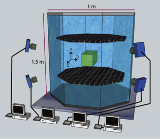
Figure 1. Experimental setup (figure reproduced from [33]). In the octagonal flow between oscillating grids, a central viewing volume in the focus of the four video cameras is illuminated by a green Nd : YAG laser.
Download figure:
Standard image High-resolution imageWe use four cameras (1280 × 1024 at 450 Hz) with a custom real-time image compression system [33, 34] to allow continuous imaging. With the two dimensional images from each of these cameras, we reconstruct the coordinates, orientations, and rotation rates of particles in three dimensions. A green Nd : YAG laser with 50 W average power illuminates a detection volume of roughly  cm3 at the center of the tank, where the flow is quite homogeneous [35]. We used two perpendicular expanded beams in the horizontal plane, each reflected back upon itself, in order to provide four directions of illumination and minimize shadowing of some arms of a particle by other arms. With an average particle number density of only
  , there was a particle in view less than 20% of the time, which made the image compression system essential for acquiring enough trajectories to converge statistics [34].
2.3. Image analysis
Orientation. An example of a jack imaged by all four cameras is shown in figure 2. When a particle is visible on all four cameras, we find the three dimensional position of the particle using stereomatching methods [36]. We developed a nonlinear fitting algorithm to determine the orientation of a particle from a set of camera images. Any orientation is specified by a rotation matrix,  , which can be parameterized by three Euler angles
  [37]. From a measurement of the particleʼs center and an initial guess of its orientation, we construct a model of the particle and project it onto each of the four image planes using the calibrated camera parameters [38]. The total difference in intensity between a model image and an experimental image provides the residual that is minimized by a nonlinear search in Euler angle space. We observe that on rare occasions, self-shadowing between arms of the particle leads to local minima which can cause errors in the measured Euler angles. Effects of orientation measurement errors on our results are discussed in the section 3.
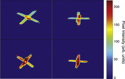
Figure 2. A sample image of a jack from each of the four cameras. The pairs of red and green asterisks denote the two ends of an arm determined by the orientation-finding algorithm.
Download figure:
Standard image High-resolution imageTo minimize computational cost, we project the endpoints of each arm onto the image plane of each camera, and then model the intensity distributions in two dimensions. The model image of an arm is formed by a Gaussian intensity distribution along the width of each arm (in 2D) and a Fermi intensity distribution across the length of the arm. For jacks and crosses, each arm in the model has an identical intensity distribution. As can be seen from figure 2, the arms in the experimental images are not of uniform intensity. The observed intensity has a non-trivial dependence on the angles between the arms, the illumination, and the viewing direction [39], which has not yet been included in our model. However, we found the simple model adequate enough for our purposes.
The orientation-finding algorithm must be seeded with an initial guess for the orientation. Except for the first frame of a track, we use the previous frame as the initial guess, since the rotation between frames is less than 0.01 radians. The initial guess for the beginning of a particle track is reliably generated using an optical tomographic reconstruction algorithm [40]. We also compared tomographic reconstruction as a method for finding particle orientation, but we found it to be both less accurate and more computationally expensive than our own algorithm.
The Euler angles found for a jack give 1 of the 24 orientations related by symmetry. To see this, consider 1 of the 6 arms of a jack and define it by the vector  ; there are 4 symmetrically identical orientations obtained by rotations of
  about the z axis. There are 4 such orientations for each of the 6 arms, for a total for 24. A cross has 8 symmetrically identical orientations, and a rod has 2. We ensure that we have a consistent series of orientations along a single trajectory by comparing the orientation found in each frame with that from the previous frame, and choose the orientation of the particle that produces the smallest total rotation between frames.
Figure 3(a) shows a representative track for a cross, which is  long. It demonstrates the effectiveness of our algorithm at determining the full range of orientations. At various points along the track, the rotation of the cross about a vector nearly coplanar with its two arms is clearly visible. In figure 3(b) we also show an example jack trajectory that is
  long.
long.
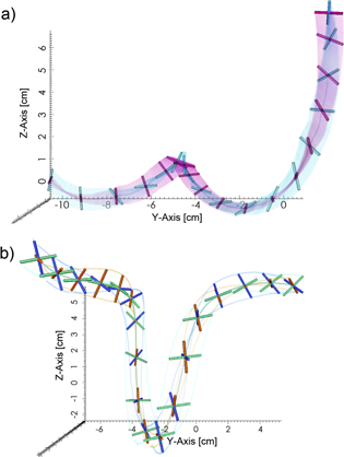
Figure 3. (a) A reconstructed trajectory of a cross in three-dimensional turbulence. The two different color sheets trace out the path of the particle through space and time. The length of the particle track is 336 frames, or  . A cross is shown every 15 frames. (b) A reconstructed trajectory of a jack in three dimensional turbulence. The three different colors distinguish the arms of the jack and trace out their path as the particle rotates. The dark green line denotes the trajectory of the jackʼs center. The length of the particle track is 1025 frames, or
  . A jack is shown every 50 frames. (Note: neither the crosses nor the jacks shown above are drawn to scale.)
Download figure:
Standard image High-resolution imageSolid-body rotation rate. Once we have measurements of orientation and position at each time step, the natural quantity to consider is the rate of change of the unit vector defining the particleʼs orientation, which we call the tumbling rate,  . For crosses and jacks, we can also measure the full solid-body rotation rate vector,
  , from a series of orientation measurements smoothed along the particleʼs trajectory. One method for doing this has been described in [29]. We take a different approach using the tools we already developed for least squares optimization in Euler angle space. The problem can be framed as finding the initial orientation matrix,
  and the finite rotation matrix over a single time step,
  , that together give the particle orientation matrix as a function of time

where τf is the period between images and ti is the time of the initial frame. A nonlinear least squares fit is used to find the six Euler angles defining the matrices  and
and  that yield the best match to the measured orientation matrices. In accordance with Eulerʼs theorem [37],
  can be decomposed as a rotation by an angle Φ about the solid body rotation axis,
  , from which we obtain the magnitude of the solid body rotation rate,
  .
.
The solid-body rotation rate,  , is related to the tumbling rate by
  . The difference between the two quantities is that
  does not depend on the vector component of
  lying along
  . We use this relationship to determine the tumbling rate from measurements of particle orientation and their solid-body rotation rate. In order to correct for the contributions from orientation measurement errors to a measurement of the mean square tumbling rate, one needs to measure
  over a a range of fit-lengths, τ
  . Figure 4 shows our measurement of
  as a function of τ. The solid lines are fits of the function

where the first term models the random error that dominates at small τ and the second term models the effect of filtering experimental measurements of orientation [32]. The fit parameter C gives an estimate of the function value at  if there were no random errors.
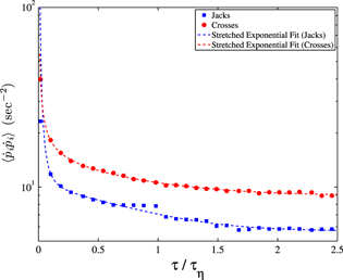
Figure 4. Measurements of the mean square tumbling rate,  , as a function of the fit length for both jacks (blue) and crosses (red). To determine the true value, we extrapolate to zero fit-length by fitting the data to a stretched exponential [32].
Download figure:
Standard image High-resolution image3. Results
From the measured solid-body rotation rates of many jacks and crosses, we can obtain the probability density function (PDF) of the squared tumbling rate, which is shown in figure 5. Also shown is the PDF obtained from direct numerical simulations of spheres [24]. All three PDFs agree within experimental uncertainties. Numerical work has shown that there should be slightly more probability density in the tail of the PDF for rods and disks than there is for spheres [24]. Within our measurement error, we cannot distinguish between the two PDFs. This is consistent with the numerical data where the mean square rotation rate differs by no more than a factor of two up to  . The error bars shown in figure 5 account for random error as well as the systematic error that results from the fit-length dependence of the tumbling rate measurements. An additional source of error that is not included in the error bars is the self-shadowing of particles as they pass through certain orientations dependent on the camera configuration. The most dramatic cases are when an entire arm is missing from each of the four cameras, such that a jack, for example, will look like a cross along part of a given trajectory. The reduction in accuracy in determining these particular orientations occasionally leads to erroneously high measurements of the solid-body rotation rate, which pushes additional probability density towards the tail of the PDF. This effect is stronger for jacks than for crosses, which may be why the jack PDF is sometimes slightly higher in our measurements at large tumbling rates.

Figure 5. The PDF of the mean square tumbling rate for our experimental measurements of crosses (red squares) and jacks (blue circles) as well as direct numerical simulations of spheres (solid line).
Download figure:
Standard image High-resolution imagePrevious work by Parsa et al showed that the mean square tumbling rate,  , for axisymmetric prolate ellipsoids is strongly affected by alignment of anisotropic particles by turbulence [24]. They found agreement between simulations and experimental measurements of rods, but particles with a wider range of aspect ratios could not be measured experimentally with the tools available at that time. We have now measured the mean square tumbling rate of crosses and jacks using the techniques described in section 2. In figure 6, we show the mean square tumbling rate normalized by the Kolmogorov timescale as a function of aspect ratio. Our measurements show crosses tumbling at a considerably higher rate than jacks or rods, but still more slowly than the randomly-oriented prediction. There is good agreement with simulations across the full range of aspect ratios, α.
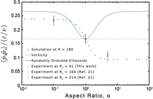
Figure 6. Mean square tumbling rate as a function of aspect ratio. Solid squares are our data for crosses and jacks. The other data is from [24]. Plus symbols are numerical simulations. The triangle and circle are experimental measurements of rods at  and 160. The solid line is an analytic result for randomly oriented axisymmetric ellipsoids.
Download figure:
Standard image High-resolution imageIn turbulence experiments, it is always a challenge to measure the energy dissipation rate, which appears in the normalization of the vertical axis in figure 6. We attempted to make independent measurements using non-fluorescent tracer particles, but did not succeed because of reduced light scattering from tracers in the density-matched CaCl2 solution. However, the measurements of jack rotations provide a new way to measure the energy dissipation rate. Because they rotate like spheres, they give a direct measurement of the vorticity, and in isotropic turbulence their vorticity is directly related to the energy dissipation through  =
= . This implies that for spheres
  [24]. We use this to determine our energy dissipation rate. This makes our jack data at
  match the simulations by definition, and the agreement of the cross data at aspect ratio
  with numerical simulations is an independent result of the measurement.
The solid green curve in figure 6 gives the mean square tumbling rate as a function of aspect ratio for randomly oriented axisymmetric ellipsoids. While the tumbling rate of jacks is unmodified from the randomly oriented case, both rods and crosses show smaller tumbling rates due to the effects of alignment by turbulence. Shin and Koch were the first to notice that the tumbling rate of rods that have correlated with a turbulent flow is reduced in comparison to that of randomly oriented rods [20]. More recent numerical work showed that the effects of alignment persist across the full range of aspect ratios [24]. The leading-order effects are contained in the Lagrangian three-point correlations of the velocity gradients, which imply higher tumbling rates for disks than for rods [19]. A number of studies on the dynamics of rods show that they align with the vorticity, and this has been used to explain the slower tumbling rate of rods since the component of the vorticity along the rod axis does not contribute to its tumbling rate [22, 23, 41, 42]. Numerical simulations of disks show that they align with their axis perpendicular to the vorticity which explains a larger tumbling rate for disks than for rods [19].
We can directly measure preferential alignment of a particle by measuring the angle between the orientation of the particle and its solid body rotation rate vector. In figure 7, we plot the PDF of the magnitude of the cosine of this angle,  , for both crosses and jacks, and compare them with numerical simulations. The peak near
  for crosses in figure 7(a) shows that disks preferentially align with
  perpendicular to
  . Figure 7(b) confirms the same story as figure 7(a). It shows that an arm of a cross is preferentially aligned with the solid body rotation rate vector. The height of the peak in figure 7(b) is lower than that in figure 7(a) because any vector in the plane of the disk is equally likely to align with
  . In a turbulent flow, disks preferentially rotate like a coin spun on its edge upon a table rather than a frisbee rotating in flight. For jacks in figure 7(c), there is no preferential alignment because they rotate like spheres. Numerics and experiment are in quite good agreement. The deviations near
  for crosses are likely the result of combined measurement error in the solid body rotation rate vector and the orientation unit vector. Our ability to resolve the peak in the PDF is limited by the measurement error in
  , which would appear as horizontal error bars in figure 7(a) and rounds off the peak. Recent numerical work has studied the preferential alignment of disks with the direction of fluid vorticity [19]. Their results are in qualitative agreement with our results on the alignment of disks with their own solid-body rotation rate.

Figure 7. The PDF of the alignment between a particleʼs orientation and its solid body rotation rate,  , for (a) crosses and (c) jacks. Symbols are experimental measurements and solid lines are numerical simulations. (b) Shows the alignment of one of the arms of a cross,
  , with its solid body rotation rate vector.
Download figure:
Standard image High-resolution image
The observed alignment in figure 7 seems natural if it is thought of as a result of the Lagrangian stretching of the fluid. Stretching will align both the vorticity and a long axis of a particle with the stretching direction, as defined by the maximum eigenvector of the left Cauchy–Green strain tensor [42]. For rods, this means that  dynamically aligns with the vorticity, since it lies parallel to the long axis of rod, and the tumbling rate is reduced. For disks, since
  lies perpendicular to any long axis,
  is expected to preferentially align perpendicular to the fluid vorticity [19]. Once they have become correlated with the turbulence, the solid-body rotation rate of disks will be dominated by the fluid vorticity and
  will be preferentially perpendicular to the solid-body rotation rate direction as well. This creates a larger tumbling rate for disks compared to rods since
  , consistent with the data in figure 6.
Although disks tumble faster than rods, they still tumble slightly slower than if they were randomly oriented, as seen in figure 6. Since disks have a much smaller difference from the randomly oriented case, one might conclude that disks are less strongly aligned than rods by the turbulence. However, this is largely a result of the way  is defined. We have measured the normalized mean square tumbling rate of a unit vector along one of the arms of a cross as
  , which is smaller than the tumbling of either crosses or jacks and the same as measurements for rods within experimental error. This explicitly indicates that crosses (disks) are also strongly aligned by turbulence, and it is only the definition of
  as perpendicular to the two arms that increases the mean square tumbling rate so much in comparison to rods. It is not easy to directly compare the degree of alignment of rods and disks because disks have an entire plane that can align with the stretching, while rods have only a director. The picture that emerges from our data and previous work is that anisotropic particles are aligning with the Lagrangian stretching direction, and this suppresses the tumbling rate, compared to the case of randomly oriented particles, for all aspect ratios except nearly spherical oblate ellipsoids. The amount of suppression is strongly dependent on the axis whose tumbling rate is considered.
4. Conclusions
We have developed a method for measuring the time-resolved Lagrangian orientation and solid body rotation rate of anisotropic particles in a turbulent flow. By measuring the rotation of 3D printed jacks and crosses we are able to extend previous measurements of rods to cover the full range of aspect ratios of axisymmetric ellipsoids. Moreover, we have provided a way to directly probe Lagrangian vorticity with a single particle measurement, which has potential for application in a wide range of flows and Reynolds numbers. We find that the mean square tumbling rate,  , agrees with DNS data on sub-Kolmogorov scale axisymmetric ellipsoids at points spanning the full range of aspect ratios. Our measurements show that crosses are preferentially aligned in turbulence with their orientation axis perpendicular to their solid body rotation rate vector. To the best of our knowledge, this is the first direct experimental measurement of the preferential alignment of particles with their rotational motion in a turbulent flow. Our results support a natural picture of alignment in turbulence where particles have their long axes aligned with the Lagrangian stretching direction of the fluid flow.
Acknowledgements
It is our pleasure to thank Jonas Einarsson, Peko Hosoi, Nadia Cheng, Bernhard Mehlig, Vikram Singh and Federico Toschi for helpful discussions. We also thank Federico Toschi and Enrico Calzavarini for providing us with the DNS data. We acknowledge support from the Wesleyan McNair program, US NSF grant DMR-1208990, and COST Actions MP0806 and FP1005.
Appendix. Resistive force theory
Resistive force theory is widely used to model the motion of slender bodies at small Reynolds number (see, e.g., [43]). We will apply it first to a small thin rod of width a and length l in a general velocity field. Then we will generalize to multiple perpendicular rods in order to show that jacks rotate like spheres and crosses rotate like disks.
Resistive force theory assumes that the differential viscous drag forces acting on a small segment of a slender body are [44]

where  is parallel to the rod, while
  is perpendicular to the rod and responsible for producing all of the torque. The constants Cd is the drag coefficient, and
  is a vector along the axis of the slender body. The vector
  is the relative velocity between the segment and the fluid, and its subscripts indicate the component parallel or perpendicular to the slender object.
We can use these expressions to calculate the total torque due to fluid flow past the rod. Since the particles are on the order of the Kolmogorov scale, we linearize the velocity field
Here and throughout the section, we will use the Einstein summation notation. Taking the center of the particle to be at rest at the origin, the velocity can be written as
where  is the normalized orientation vector of the rod and r is the radial distance from the center of the rod. The drag force is determined by the relative velocity between the fluid and the rigid-body rotation of the rod

The torque comes from the component of velocity perpendicular to the rod,  . We can write this by subtracting the parallel component from the full relative velocity. Entering
  into equation (A.1), we have
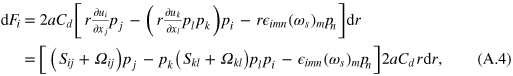
where we have written the velocity gradient in terms of its symmetric and antisymmetric parts, Sij and Ωij, respectively.
We now rearrange (A.4), noting that  since
since  forms a symmetric tensor while Ωkl is antisymmetric, and compute the differential torque element
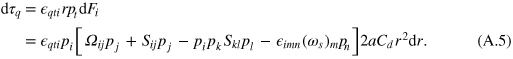
Integrating along the length of the rod, l, we have the total torque
Now, consider the term  . This is nothing else than the rate at which the orientation of the rod is changing,
  . Thus, we have

For any orientation,  , (A.7) can be used to compute the qth component of the torque on a single rod. For Stokes flow

When we impose this constraint on (A.7), we immediately recover Jefferyʼs equation (equation (1)) in the limit of infinite aspect ratio (i.e., for a rod)

With this established, we can now explore the rotational dynamics of objects that are composites of perpendicular rods with arbitrary lengths. From (A.6), we can read off the qth component of the torque on the αth arm,  . The total qth component of the torque is then

where  is the number of arms on the particle,
  is the length of the αth arm, and
  is the pre-factor for the αth arm,
  . From here, we can extend the calculation made for single rods to particles composed of N rods. The zero net torque condition of Stokes flow still holds true, but there will now be contributions from multiple arms because of the sum over α. If we consider axisymmetric particles,
  , and are careful to define
  along the symmetry axis of the particle, equation (A.10) leads to an analog of Jefferyʼs equation (1)
where  .
.
We find that resistive force theory for the rotational motion of a set of three perpendicular rods with  reproduces Jefferyʼs equation (1), except that the aspect ratio appears with cubic dependence rather than quadratic, such that the particles behave like ellipsoids with an effective aspect ratio [26]. The cases we study are jacks,
  with
with  , and crosses,
  but
but  with
with  . These both happen to be cases where
  , so, within the limits of resistive force theory, we can simply say that jacks rotate like spheres and crosses rotate like disks.