


Abstract
We report on a theoretical study of a dz2 surface state at the tungsten (110) surface, addressing in detail the spin-resolved electronic structure as well as photoemission spectroscopy. In agreement with recent experiments, this surface state shows a strongly anisotropic dispersion: in the  –
– –
– direction of the surface Brillouin zone, it disperses linearly but becomes flattened along the
  –
– –
– direction. The ab initio calculated spin texture agrees with the one derived from a model Hamiltonian; due to twofold surface symmetry and time-reversal symmetry, the out-of-plane spin polarization vanishes. The photoemission intensities depend sensitively on the polarization of the incident light, because of the orbital composition of the surface state. The photoelectrons become spin-polarized out-of-plane, which is attributed to breaking the time-reversal symmetry by the excitation process.
Export citation and abstract BibTeX RIS

Content from this work may be used under the terms of the Creative Commons Attribution-NonCommercial-ShareAlike 3.0 licence. Any further distribution of this work must maintain attribution to the author(s) and the title of the work, journal citation and DOI.
1. Introduction
Topological insulators are a class of materials whose properties are important for both fundamental physics and device applications (e.g. [1]). While insulating in the bulk, these solids show surface states with unique features: they bridge the fundamental band gap and show linear dispersion, similar to relativistic massless particles. The two branches of such a surface state that are related by time-reversal symmetry cross at a time-reversal invariant momentum [2]; this crossing point in energy E and momentum ℏk is called a Dirac point. The spin–orbit interaction prescribes a specific spin texture of the Dirac surface states [3].
Inspired by the ground-breaking early investigations, mainly on HgTe systems [4] and bichalkogenides (e.g. Bi2Se3) [5], there is now an ongoing search for new topological insulators [6]. Means of transforming conventional insulators into topological insulators are, for example, lattice distortions [7] or substitutional disorder [8]. This quest has led also to the re-inspection of the surface states of materials that were believed well investigated and understood but cannot be transformed into a topological insulator: transition metals such as W(110) [9].
Recently, a surface state has been found on W(110) whose dispersion shows striking similarity to that of a Dirac surface state [9]. This finding is particularly astonishing since W(110) misses almost all ingredients of a true topological insulator (e.g. of the bichalkogenide type). (i) It is a metal and, thus, shows no fundamental band gap. However, it displays gaps in parts of the Brillouin zone below the Fermi energy. (ii) A band inversion across a fundamental band gap is missing. (iii) It is not a compound, in contrast to the topological insulators of the HgTe and Bi2Se3 types. (iv) The energy range of the observed surface state is populated by d electrons, in contrast to p electrons at the fundamental band gap in topological insulators. However, topological insulators and tungsten have in common a strong spin–orbit coupling: Z = 74 for tungsten (Swedish for 'heavy stone').
The 'Dirac surface state'4 on W(110) is energetically situated in a partial band gap that is due to spin–orbit coupling, similar to the spin–orbit-induced fundamental band gap in a topological insulator. It shows a band crossing with linear dispersion, that is a Dirac point. However, while true Dirac states form a—more or less—isotropic two-dimensional electron gas (for warping of Dirac states see [3, 10]), the Dirac state of W(110) is highly anisotropic: in one direction of the two-dimensional Brillouin zone, it disperses linearly and strongly but becomes 'flattened' along the orthogonal direction. This finding is explained by the twofold symmetry of the W(110) surface [11].
It turns out that, to our knowledge, this special surface state has so far been investigated experimentally by means of spin- and angle-resolved photoelectron spectroscopy (SARPES) and by a model calculation [9, 11]. However, a comprehensive theoretical study by means of first-principles electronic structure calculations is missing. In this paper we report on such a theoretical investigation.
We show that all features of the Dirac state can be explained by the Rashba spin–orbit coupling [12, 13]. Our first-principles calculations predict a second surface state with lower binding energy and opposite spin polarization with respect to the Dirac state. The hybridization of the Dirac state and the surface state results in a maximum in the dispersion of the Dirac state that, as a consequence, does not bridge the band gap. These observations are similar to those in the Rashba systems Bi/Ag(111) [14] and Bi/Cu(111) [15]. There, the spz surface state hybridizes with a pxpy surface state at higher energy and also opposite spin polarization [16]. In Bi/Cu(111), this hybridization even results in a spin reversal [15]. The spin polarization is entirely in-plane, as is explained by symmetry considerations.
In photoemission experiments, Miyamoto et al [11] found a strong dependence of the photoemission intensities on the light polarization. This feature has been convincingly explained by the orbital composition of the Dirac state. Nevertheless, such a finding calls for support by first-principles photoemission calculations that provide a direct link between the electronic structure calculations for the ground state and the experiments. Hence, we performed such computations within the relativistic one-step model of photoemission and confirm the experimental findings. On top of this, we address the spin polarization of the photoelectron and compare it with that of the Dirac state, using the experimental setups. It turns out that the photoelectron's spin can be tilted out-of-plane, although the spin of the Dirac surface state is in-plane; this finding is attributed to time-reversal breaking by the photoemission process.
The paper is organized as follows. Theoretical aspects are addressed in section 2. The results-and-discussion (section 3) comprises the analysis of the dispersion (section 3.1), the spin texture (section 3.2), as well as the spin- and angle-resolved photoemission (SARPES, section 3.3). Concluding remarks are given in section 4.
2. Theoretical aspects
In this section, we address the model Hamiltonian that is used for analyzing the basic properties of the Dirac state (section 2.1). Further, we give details on the first-principles electronic structure (section 2.2) and photoemission calculations (section 2.3).
2.1. Model Hamiltonian
Rashba-split surface states are well described by model Hamiltonians (see [3, 17] for Au(111) and bichalkogenide topological insulators, respectively). For the W(110) surface, we derived an analogous Hamiltonian from k·p perturbation theory [18], taking into account the twofold symmetry of this surface (point group 2mm [19]). This Hamiltonian agrees with that derived by Miyamoto et al [11]. The model Hamiltonian

comprises three terms. (i) H0(k) describes the basic dispersion of an anisotropic two-dimensional electron gas without spin–orbit coupling,

The effective masses m☆y and m☆x are −4.7me and 3.3me, respectively (electron mass me; all parameters in this section have been taken from [11]). (ii) H(1)soc(k) is the Rashba-type spin–orbit Hamiltonian in first order in the wavenumbers kx and ky,

with Pauli matrices σx and σy (αx = −0.08 eV Å and αy = 1.05 eV Å). (iii) The contribution of third order to the spin–orbit coupling is given by

(αx3 = 5.57 eV Å3, αx2y = 12.3 eV Å3, αxy2 = −25 eV Å3 and αy3 = 1.13 eV Å3).
The above Hamiltonian reveals considerable differences with respect to those for systems with (111) surfaces [20, 21]. The latter surfaces show threefold rotational symmetry; their point group 3m (cf Au(111), Bi/Ag(111) and Bi2Te3(111)) implies αx = −αy = αR (Rashba parameter). Also the warping introduced by the third-order terms depends only on a single parameter [3]. Further, it tilts the spin polarization of the surface states out of the surface plane, as is described by the Pauli matrix σz. For a system with point group 2mm, the two mirror planes that are perpendicular to each other allow, in principle, for an out-of-plane tilt. However, time-reversal symmetry forbids this because E(k,s) = E(−k,−s); compare the actions of C2z and T on the spin vector s in table 1 which dictates sz ≡ 0. Hence, the spin polarization vector s has to be in-plane for all wavevectors and H(3)soc(k) comprises only terms with σx and σy. Furthermore, for a wavevector parallel to the kx-axis, the table yields sx ≡ 0; thus, on the  –
– –
– line of the two-dimensional Brillouin zone (figure 1), only sy is nonzero. Analogously, for k along the ky-axis, one obtains sy ≡ 0, which implies a nonzero sx along the
  –
– –
– –
– –
– . These impositions are fully supported by our first-principles calculations.
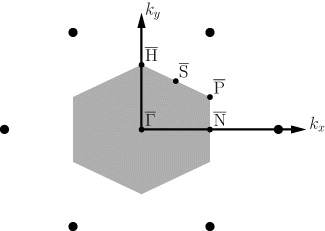
Figure 1. Reciprocal lattice of the W(110) surface. Lattice points are given by large filled circles. The first Brillouin zone is displayed in gray, with its high symmetry points marked by small filled circles. The kx and the ky axes are invariant under reflections mxz and myz, respectively (see table 1).
Download figure:
Standard imageTable 1. Effect of symmetry operations of the point group 2mm and of time reversal on the wavevector k = (kx,ky), the spin vector s = (sx,sy,sz) and the vector potential A = (Ax,Ay,Az) of the incident light (in photoemission). See also figure 1.
| 1 | kx | ky | sx | sy | sz | Ax | Ay | Az | Identity |
| mxz | kx | −ky | −sx | sy | −sz | Ax | −Ay | Az | Reflection at xz plane |
| myz | −kx | ky | sx | −sy | −sz | −Ax | Ay | Az | Reflection at yz plane |
| C2z | −kx | −ky | −sx | −sy | sz | −Ax | −Ay | Az | z-rotation about π |
| T | −kx | −ky | −sx | −sy | −sz | Ax | Ay | Az | Time reversal |
This single-band approach leads to agreement of model and experiment in the energy region close to the Dirac point (band crossing at kx = ky = 0,  ). However, it does not hold at higher energies where—as we shall show below—the Dirac state hybridizes with another surface state (see also [15, 16]).
2.2. First-principles electronic structure calculations
We have performed ab initio calculations within the framework of the local density approximation to density functional theory. The electronic properties have been obtained by multiple-scattering computations with a relativistic layer Korringa–Kohn–Rostoker (KKR) code [22, 23]. Spin–orbit coupling is fully accounted for by solving the Dirac equation. The exchange-correlation functional is taken from [24].
The layer-resolved Green function Gll(E + iη,k) provides detailed information on the electronic structure. l is the layer index, E the energy, η a small offset from the real energy axis and k = (kx,ky) is the in-plane wavevector. Both orbital composition and spin texture of the electronic states have been obtained from the spectral density [25]

by taking appropriate partial traces. A comparison of Nl(E,k) for different layers l at fixed (E,k) gives the localization of the surface states in the vacuum–surface region.
The spin textures of the electronic states are addressed by means of spin differences s↑μ − s↓μ that are obtained from the spectral density in (5). The spin projections ↑ and ↓ are given with respect to the chosen spin quantization axis μ (e.g. μ = y for k on the kx-axis).
The entire system comprises three regions: (i) semi-infinite bulk, (ii) the surface region that consists of six W layers and four layers of vacuum and (iii) semi-infinite vacuum. The image potential barrier is mimicked by the so-called empty muffin-tin spheres, rather than by a smooth interpolating function [26]. In a KKR calculation of the surface electronic structure of W(110) by Giebels et al [27], a smooth interpolating function is used as an image-potential barrier. We find no significant changes with respect to our calculation that uses empty muffin-tin spheres. The only exception is a slightly better binding energy of the Dirac surface state in that calculation because of the adjustment of the barrier parameters. All other properties, in particular the spin polarization, agree very well. Bulk layers are denoted  , whereas surface layers are named
  ,
,  ,
,  , etc, starting with the topmost surface layer
  . Similarly, vacuum layers are
  ,
,  , etc. The surface layer is relaxed toward the bulk by δd12 = −2.75% of the bulk interlayer distance, as has been obtained from the surface x-ray diffraction [28]. Low-energy electron diffraction (LEED) gives comparable contractions (e.g. −2.2% in [29]).
The layer KKR method relies on two representations for the electronic states: plane waves and spin-angular functions. The number of plane waves, used in the interlayer scattering, was at least 50. The maximum angular momentum, used in the single-site scattering and the intralayer scattering, was lmax = 3. Both numbers guarantee converged results. The offset η from the real energy axis in (5) is 5 meV.
2.3. Photoemission calculations
We have also computed spin- and angle-resolved photoemission intensities within the relativistic one-step model of photoelectron spectroscopy [22, 30], using the potentials of the first-principles calculations as input. These theoretical spectra provide a direct link between the spectral density maps of the initial states (occupied states) and the measured intensity maps of the photoelectrons.
The spin-density matrix of the photoelectron is calculated from

which represents the triangular Feynman diagram of the one-step model of photoemission [31, 32]. The initial (occupied) electronic states are represented by the Green function G(E − ℏω,k). The dipole operator Δ(ω)∝α·A(ω) mediates the transition from the initial state to the outgoing photoelectron state, that is the time-reversed LEED state Φσ(E,k) with spin projection σ. α is a vector of Dirac matrices [33], while A(ω) is the vector potential of the incident radiation with photon energy ℏω.
The spin-averaged photocurrent is given by I(E,k) = tr ρ(E,k), while the spin polarization of the photoelectrons reads

(σ is the vector of Pauli matrices). Due to spin–orbit coupling, the photocurrent is, in general, spin polarized even for nonmagnetic samples, depending on the specific setup (see [34] and references therein).
The above model takes into account the correct boundary conditions [35], the electronic structure above the vacuum level (via the time-reversed LEED state), dipole selection rules (via the dipole operators) and the electronic structure of the occupied states. The in-plane wavevector k is conserved due to translational invariance within the layers. Hence, it allows for quantitative comparison with experiments (see e.g. [17, 36]).
The photoemission calculations use the same setup as the electronic structure calculations. The Green function in (6) introduces a sum over all layers [37] which is approximated by a finite sum over the outermost layers. This is justified by the finite lifetime of the photoelectrons that introduces the surface sensitivity of photoelectron spectroscopy in the vacuum ultraviolet (VUV) range [38]. Here, the topmost 30 layers contribute to the photocurrent. The lifetime broadening is mimicked by an imaginary part of the energy, taken as −0.025 eV for the occupied and −1.0 eV for the unoccupied states. These values are chosen to clearly show the spin texture of the Dirac-like surface states. However, for reproducing experimental spectra these values have to be optimized and have to be taken as energy dependent. The quality of our approach may be judged from the data shown in [36].
The setup is adopted from [9, 11] (see figure 1 in these publications). The optical plane is spanned by the surface normal, the direction of light incidence and the direction of photoelectron detection. The sample is rotated about the surface normal by an angle ϕe and the photoelectrons are detected at a polar angle θe. The polar angle θph of light incidence is 50°. We use both completely s- and p-polarized light with a photon energy of 22.5 eV (as in the experiment).
3. Results and discussion
3.1. Dispersion
In the energy range that is relevant for the Dirac-like surface state, the W band structure shows a pocket-shaped partial band gap that is induced by spin–orbit coupling (top row in figure 2). This band gap is occupied by a strongly dispersive bulk band in the vicinity of the Brillouin zone center  . As we will see below, also a strongly dispersive surface state follows its band edge.
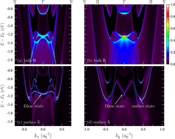
Figure 2. Spectral density of a bulk layer  (top row) and the topmost surface layer
  (bottom row) along the
  –
– –
– (left column) and the
  –
– –
– –
– –
– (right column) lines of the two-dimensional Brillouin zone. The spectral densities are normalized and, thus, share a common color scale (right of panel (b)). The Dirac state and a surface state are marked by arrows. The wavenumber k is given in inverse Bohr radii, a−10.
Download figure:
Standard imageAt an energy of −1.25 eV, an M-shaped region with a high spectral density shows up around  . Along the
  –
– –
– the dispersion is concave (bent upward, figure 2(a)) whereas along the
  –
– –
– there is, in addition to the concave shape, a very small convex region (bent downward, figure 2(b)) very close to
  . This anisotropy has consequences for the dispersion of the Dirac-like surface state that is split off this bulk band.
Considering the spectral density of the topmost surface layer  , we find a surface state at −1.15 eV (experiment: about −1.2 eV), whose concave and weak dispersion follows that of the associated bulk band edge (this Dirac state is marked by an arrow in figure 2(c)). Along the
  –
– –
– , its dispersion becomes linear and much stronger than along the
  –
– –
– . It is this finding that is clearly reminiscent of the Dirac state in a topological insulator, say Bi2Se3. Due to the strong anisotropy of the dispersion, however, we can hardly speak of an isotropic Dirac cone.
When deliberately changing the inward relaxation δd12 of the top W layer  to zero, the Dirac point is shifted into the bulk band region at lower energies. This behavior is typical for a Shockley surface state that occurs due to a change of the crystal potential at the surface (rather than to a simple truncation of the infinite bulk system). From this finding we conclude that the surface relaxation is not essential for the appearance of the Dirac surface state. However, the inward relaxation 'pushes' the Dirac point into the bulk band gap. Hence, other heavy bcc(110) surfaces may show Dirac surfaces states as well.
As has been found in the experiment by Miyamoto et al, the Dirac state does not cross the band gap but displays a sharp maximum at k = ± 0.2 a−10 and E = −0.86 eV (figure 2(d)). This change from an upward to a downward dispersion is explained by the strongly dispersive surface state that is associated with the bulk band edge mentioned above (marked 'surface state' in the figure). Both states belong to the same irreducible representation of the small group of k and, therefore, cannot cross. Their small distance in (E,k) results in a sizable hybridization which we will discuss by means of surface localization now.
The spectral densities of the surface states become blurred when they appear in a region of bulk states, an indication of hybridization of surface and bulk states [39]. Another manifestation of hybridization but among surface states is their surface localization. Close to the Brillouin zone center  , the Dirac state shows largest spectral weight in the topmost layer (filled triangles at layer
  in figure 3) and decays monotonously toward the bulk without modulation. At larger wavenumbers, the Dirac state and the strongly dispersive surface state hybridize (figure 2(d)). As a consequence, they show similar properties: the spectral densities of these states, for example, are largest at layer
  with almost identical size. However, their decay toward the bulk is slightly modulated, in contrast to the Dirac state at
  .
.
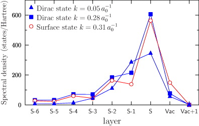
Figure 3. Surface localization of the Dirac state (blue filled symbols) and a surface state (red open circles). The energy is E = −1.07 eV; the wavevector is along the  , with the wavenumber k indicated for each state in inverse Bohr radii (see figure 2(d)).
  is the topmost surface layer;
  indicates vacuum layers.
Download figure:
Standard imageThe linear dispersion of the Dirac state along  –
– –
– mimics that of a massless fermion. Along the
  –
– –
– this state becomes 'massive', that is, it exhibits parabolic dispersion. Hence, this strong anisotropy could be used to gradually increase or decrease the effective electron mass by changing the azimuth of the wavevector k.
To elucidate the anisotropy of the dispersion in more detail, we present constant energy contours (CECs) of the spectral density in the surface layer  at selected energies (figure 4). At −1.0 eV, the Dirac state shows up as the inner rhombus that is elongated along kx (the
  –
– –
– ; figure 4(a)). This finding illustrates the weak dispersion in kx and the strong dispersion in ky. Due to the maximum in its dispersion (figure 2(d)), the Dirac state manifests itself in the CEC also as the innermost oval (indicated by an arrow as well). The strongly dispersive surface state shows up as the second innermost oval whose curvature follows closely that of the Dirac state. As a consequence, these states hybridize sizably in all k directions.
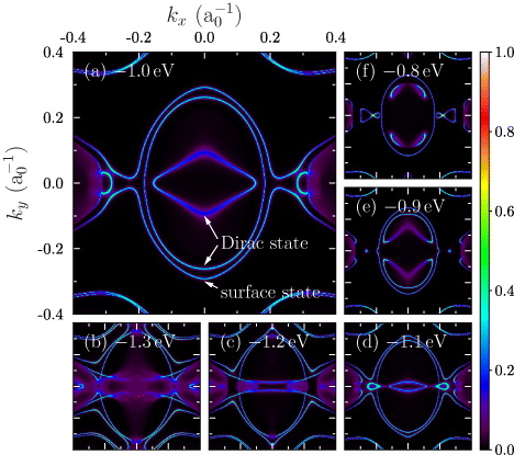
Figure 4. Spectral density in the topmost surface layer  around the center of the two-dimensional Brillouin zone for selected energies (relative to the Fermi energy, indicated in each panel). kx is along the
  –
– and ky is along the
  –
– . The Dirac state and a surface state are marked by arrows in (a). The spectral densities are normalized and share a common color scale. All panels display the same region of the two-dimensional Brillouin zone, although (a) is enlarged.
Download figure:
Standard imageThe anisotropy of the Dirac state's dispersion shows the importance of the third-order terms in the model Hamiltonian. It becomes even enhanced at lower energies, as is evident from the extremely elongated rhombus at −1.1 eV (figure 4(d)). Below the Dirac point but still above the bulk band region, for example at −1.2 eV, it appears that the spectral density shows weight only along kx; see the almost parallel lines in figure 4(c). At even smaller energies, the hybridization of the Dirac state and bulk states results in a blurred spectral density (figure 4(b)).
At higher energies, a band gap opens up in the Dirac state along the  –
– –
– (cf −0.9 eV in figure 2(c)). This opening has the consequence that the Dirac state's rhombus and oval transform into two chevron-shaped features (figure 4(e)) that lie mirror symmetric with respect to the
kx-axis.
(cf −0.9 eV in figure 2(c)). This opening has the consequence that the Dirac state's rhombus and oval transform into two chevron-shaped features (figure 4(e)) that lie mirror symmetric with respect to the
kx-axis.
A comparison with experimental ARPES data, figure 3 in [11], establishes agreement with our calculations concerning the shape of the Dirac state's rhombohedral structure in the CECs. However, the ARPES measurements do not 'illuminate' the complete shape of the rhombus which is attributed to dipole selection rules in the photoemission process. Similar findings are reported by Winkelmann et al [36]. We will address this observation in section 3.3.
3.2. Spin texture
The Rashba spin–orbit coupling implies a specific spin texture of the surface states. For an isotropic two-dimensional electron gas, the Rashba Hamiltonian yields a spin alignment within the confinement plane (here: xy or surface plane) and normal to the wavevector k. For systems with threefold rotational symmetry, a tilt of the electron spin out-of-plane has been found: small for Au(111) [17] but as large as 45° for Bi2Te3 [40]. For W(110), however, the two orthogonal mirror planes in conjunction with time reversal forbid such an out-of-plane tilt (see section 2.1). Consequently, we focus on spin differences s↑μ − s↓μ for an in-plane spin quantization axis normal to k (figure 5).
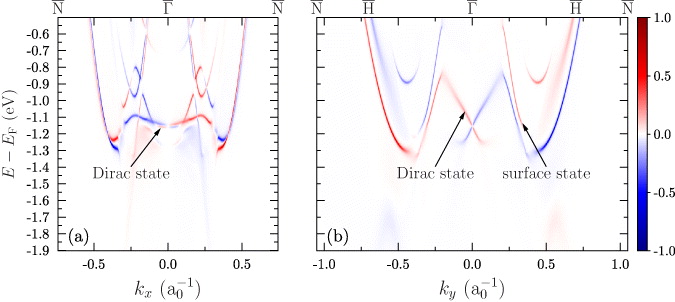
Figure 5. Spin-resolved electronic structure of the topmost surface layer  of W(110) along the
  –
– –
– (a) and the
  –
– –
– –
– –
– (b) lines of the two-dimensional Brillouin zone. The normalized spin differences s↑μ − s↓μ are given as color scale (right of panel (b)); the spin quantization axis μ is in-plane and normal to the wavevector. The Dirac state and a surface state are marked by arrows.
Download figure:
Standard imageThe Dirac state exhibits the expected spin texture that fully agrees with that derived from the model Hamiltonian. Interestingly, the strongly dispersive surface state that hybridizes with the Dirac state has a spin orientation opposite to that of the Dirac state (figure 5(b)). The degrees of spin polarization of the Dirac state are as large as 87.5% at k = 0.05 a−10 and 95.9% at k = 0.28 a−10 at E = −1.07 eV (i.e. at the (E,k) points used in 3); the surface state's spin polarization equals 86.8% at k = 0.31 a−10.
A similar observation has been made for the surface states in Bi/Cu(111) [15] and Bi/Ag(111) [16]. In these surface alloys, the Bi atoms induce two sets of surface states, one at lower energy of mostly spz orbital composition and another one at higher energy with pxpy orbital composition. The outer branch of the lower set hybridizes with the inner branch of the upper set, both showing opposite spin polarization. For W(110), the strongly dispersive surface states play the role of the upper branch. The other electronic states at the surface are as well spin polarized due to spin–orbit coupling [41, 42].
Our findings reported so far corroborate the experimental observations and the conclusions drawn by Miyamoto et al [9, 11]. In particular, they support the surface origin of the spin-resolved properties. In turn, they contrast with a recent finding by Rybkin et al [43]: in their study on W(110), the spin-polarized features were attributed to bulk origin.
3.3. Spin- and angle-resolved photoelectron spectroscopy
Having analyzed the Dirac state in the previous sections, we now address how its properties manifest themselves in the photoemission intensities. Without spin–orbit coupling, electronic states are either even or odd with respect to mirror operations. With spin–orbit coupling, however, these components become mixed in the respective double group [19]. Furthermore, even spin-up orbitals can hybridize with odd spin-down orbitals and vice versa, as has been found in Bi/Cu(111) [15]. As a result, the spin polarization is less than 100%. Since the spatial character of the initial state in the photoemission process can be selected by the polarization of the incident light, one could observe a reversal of the spin texture upon changing from s-polarized light to p-polarized light.
We will now address this effect for the  –
– –
– azimuth. For s-polarized light, the vector potential A of the incident light lies parallel to the surface plane and normal to the yz plane. Hence, only Ax is nonzero and A is odd under myz (table 1). Therefore, only odd orbitals under myz can be probed. For p-polarized light, A is even under myz and even orbitals are probed.
The spectral-density calculations yield that the Dirac state near  is mainly of dz2 orbital character which is even under myz. Consequently, its photoemission intensity is large for p-polarization (figure 6(a)) and small for s-polarization (c). As suggested before, we find the expected spin reversal: the Dirac state at ky > 0 is spin-up (blue in figure 6(e)) for p-polarization but spin-down (red in figure 6(g)) for s-polarization. As found already in figure 5(g), the highly dispersive surface state shows a spin polarization opposite to that of the Dirac state.
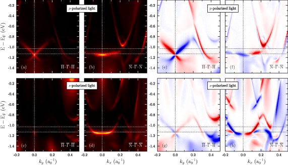
Figure 6. Spin-integrated (a)–(d) and spin-resolved (e)–(h) photoemission intensities from W(110) along the  –
– –
– and
and  –
– –
– . The polarization of the incident light is shown for each panel. Blue and red indicate opposite (in-plane) spin directions. The maximum degrees (darkest blue) are 86% (e), 33% (f), 92% (g) and 76% (h); the minimum degrees of spin polarization (darkest red) are −88% (e), −98% (f), −94% (g) and −76% (h).
Download figure:
Standard imageAnalogous considerations hold for the  –
– –
– azimuth (figures 6(b) and (d)). Similar to the
  –
– –
– azimuth, the strongly dispersive surface state is observed for p-polarized light but is absent for s-polarized light, which implies that this state is even with respect to the mirror operation mxz. The flattened states shown along kx consist of even and odd states. For p-polarized light, the flattened states show a larger intensities near the center of the Brillouin zone and fade out for larger k. The situation is reversed for s-polarized light: intensities are weaker close to the center of the Brillouin zone and become stronger for larger momenta.
The experiments by Miyamoto et al [11] reveal a rather strong sensitivity of the Dirac state's intensity on the electron detection direction: for negative k (along  –
– –
– ), the Dirac state shows up clearly but is suppressed for positive k (cf state S1 in figure 2(a) of their publication). Our computations do not show such a strong asymmetry, a finding that is easily understood from the Dirac state's orbital character (mostly dz2). To resolve this issue, we would like to suggest detailed experimental and theoretical investigations that include a spin analysis of the photocurrent.
The spin polarization of the Dirac state lies within the surface plane of all k, as is shown in the previous section. The complete in-plane spin polarization of the (initial) Dirac surface state is due to the joint effect of rotation and time-reversal invariance. The photoemission process, however, breaks the time-reversal symmetry; as a consequence, the restriction induced by time reversal on the spin polarization (operation T in table 1) is no longer valid, and the out-of-plane component of the photoelectron's spin polarization can be nonzero for k that do not lie within a mirror plane.
To investigate the out-of-plane spin component that is induced by the photoemission process itself, we have computed spin-resolved ARPES maps at constant energies (figure 7). The intensities have been obtained for polar-angle scans, with the azimuth running from −90 ° to +90 °; this is the setup as sketched in figure 1 of [9].
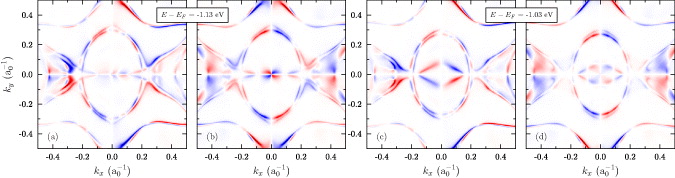
Figure 7. Spin-resolved photoemission intensities from W(110) at constant initial energies, as indicated. Panels (a) and (c) ((b) and (d)) show results for p-polarized (s-polarized) light. The red–white–blue color scale represents negative–zero–positive out-of-plane spin differences sz for polar scans in the azimuth range from −90 ° to +90 °. The maximum degrees of spin polarization (darkest blue) are 55% (a), 62% (b), 66% (c) and 65% (d). The minimum degrees of spin polarization (darkest red) are the same values but with opposite sign, due to the symmetry of the setup.
Download figure:
Standard imageFor both light polarizations, sz vanishes in a mirror plane of the surface (see table 1). However, the spin-resolved intensity patterns of s- and p-polarized light differ in their symmetry. For s-polarized light, sz shows twofold rotational symmetry (figures 7(b) and (d)); by crossing a mirror plane, it changes sign (the same holds for the in-plane spin polarization (not shown)). However, for off-normally incident p-polarized light (figures 7(a) and (c)), the twofold symmetry is broken but sz changes sign when turning ky into −ky for fixed kx. This result is fully in line with table 1 (cf the effect of the operation mxz on sz). Also the in-plane components sx and sy comply with table 1. The out-of-plane spin polarization is as large as 92% at k = (0.004,0.008) a−10 in figure 7(b) and 44% at k = (0.098,0.044) a−10 in figure 7(c). Note that these numbers depend on the chosen lifetime broadening; a larger lifetime broadening would reduce these values. We conclude that if a spin polarization component is not forbidden by symmetry it is actually nonzero. Evidently, its degree and sign depend on the transition matrix elements that are calculated from realistic initial and final states and consequently depend on the specific setup.
We would like to emphasize that the purpose of the present SARPES calculations is to show the major effects concerning the spin polarization of photoelectrons excited from the Dirac surface state. For this reason we used the setup detailed in the publications by Miyamoto et al [9, 11]. Nevertheless, we performed additional photoemission calculations using different setups: with fixed incidence angles of 20° and 50° with respect to the sample. To check the effect of the final states, we performed calculations for different photon energies as well. As a result in both cases, the photoemission intensities from the Dirac surface state and its out-of-plane spin polarization change.
4. Concluding remarks
The dz2 surface state in W(110) shows a rich variety of features which are brought about by the spin–orbit interaction. Although most of its properties that have been determined experimentally by photoelectron spectroscopy [9, 11] are explained in the present theoretical investigation, there remain a very few issues to be solved in future studies. For example, the strong asymmetry of the experimental photoemission intensities is not fully supported by our calculations. On the other hand, the out-of-plane spin polarization that is brought about by the photoemission process itself calls for an experimental investigation by spin-resolved photoelectron spectroscopy.
The observation of a Dirac-like surface state at a metal surface opens another 'playground' for spin–orbit-induced phenomena, besides the well-understood surface alloys on Ag(111) and Cu(111) (e.g. Bi/Ag(111) [14]) and the emerging field of strong topological insulators.
Acknowledgments
We are very grateful to M Donath (U Münster) and R Feder (U Duisburg-Essen) for stimulating and fruitful discussions.
Footnotes
- 4
Although W is not a topological insulator and, hence, its surface state cannot be topologically protected (that is a 'true Dirac state'), we shall call this surface state deliberately a 'Dirac state' in this paper.