Angular dependence of resistance and critical current of a Bi-2223 superconducting joint

We fabricated a Bi-2223 closed-loop sample with a superconducting joint shown in figure 1(a). A 1.6 m long Ni-alloy-reinforced Bi-2223/Ag tape (DI-BSCCO^® Type HT-NX [2, 4, 46, 47]) was used. The width and thickness of the tape were 4.5 and 0.25 mm, respectively. The reinforcement at both ends, approximately 0.2 m long, was removed [26]. A praying-hands-type superconducting joint was formed to connect both ends using a previously reported process [17, 20, 45].

To form the superconducting joint, a polycrystalline Bi-2223 intermediate layer was synthesized via heat treatment. As described in our previous study [45], during heat treatment, the sample was a one-turn loop with an approximately 0.6 m long temperature transition zone. The joint was inserted into a tube furnace and heat-treated, whereas the loop part with the reinforcement was placed outside the furnace and held at room temperature. After the heat treatment, the one-turn loop was wound into a three-turn loop with a diameter of 100 mm. The L of the sample was 1.4 μH, which was measured at room temperature before the ends were connected [42].

Current decay was measured by rotating the sample incrementally. The angle of the magnetic field (θ) was determined as shown in figure 1(b). The direction of the magnetic field at θ = 90° was parallel to the tape surface. The time dependence of the voltage of the Hall sensor (V_Hall) in the current sensor was measured at each angle. I_loop was calculated from V_Hall using a linear relationship between a current and V_Hall obtained experimentally beforehand [20, 30].

In a preliminary experiment, I_cj reached the maximum at 90°. We started to rotate the sample (decrease θ) from 90° at the experimental time (t_exp) of 0. At each angle, t was the elapsed time from when we started sample rotation. The measurement sequence, schematically shown in figure 2, is described as follows:

• (1)  
  The temperature of the sample was controlled to be 4 K.
• (2)  
  A magnetic field (B) of 0.15–0.28 T was applied to the joint at 90°.
• (3)  
  An I_loop of 220–221 A was introduced to the sample.
• (4)  
  We waited until the initial current-sharing effect in the sample became negligible and the time variation V_Hall became flat, which required several tens of minutes.
• (5)  
  The sample was rotated (θ was decreased) by 5° within 1 s while the I_loop flowed. At t_exp = 0, the sample was rotated from 90° to 85°. This point corresponded to t = 0 at 85°.
• (6)  
  The time dependence of V_Hall was measured for approximately 10 min.
• (7)  
  The 5° rotation and the 10 min measurement were repeated until θ = 0.

Zoom In Zoom Out Reset image size

Using the measured V_Hall, we obtained the time dependence of I_loop (I_loop–t) for approximately 10 min at each angle. Because we measured V_Hall at a sampling rate of 1 Hz, there were typically more than 600 data points in each I_loop–t curve.

To evaluate R_j and I_cj at each 5°-incremental angle between 0 and 85°, we used 300 data points of the I_loop–t curve at 300 s ⩽ t ⩽ 600 s. At 90°, R_j was evaluated using 300 data points at −300 s ⩽ t_exp ⩽ 0.

The value of R_j was obtained by fitting the data points of the I_loop–t curve to equation (1) using the least squares method. The value of I_cj was estimated using the I_loop dependence of the voltage (V) obtained from the I_loop–t curve. When current decay was observed, we could calculate V using equation (2) as follows:

$$\begin{equation}V = - L\frac{{{{\Delta }}{I_{{\text{loop}}}}}}{{{{\Delta }}t}}.\end{equation} \tag{ 2 }$$

The I_loop dependence of the calculated voltage (V–I_loop) was smoothed using a 15-point moving average. The smoothed V–I_loop curve at a voltage ranging from 10⁻⁷ to 10⁻⁹V was fitted to an empirical power law model (V = α I_loop ⁿ , where α and n are constants) using the least squares method. We estimated I_cj at a voltage criterion (V_c) of 10⁻⁸V, which corresponded to the I_loop value at V = 10⁻⁸V. Some of the I_loop values at 10⁻⁸ V were estimated by the extrapolation from the fitting.

Figure 3 shows V_Hall as a function of t_exp at 4 K and 0.25 T. The inset shows the magnified view at approximately 70°. From 90° to 75°, a decrease in V_Hall with time was not clearly observed; that is, V_Hall–t_exp at each angle was almost flat. This implies that the decay of I_loop was negligible at 75–90°, and the I_loop was considerably lower than I_cj. By contrast, at angles less than 75°, a decrease in V_Hall over time was evident.

Zoom In Zoom Out Reset image size

The value of V_Hall increased by less than 1 mV for each 5° rotation, as shown in the inset of figure 3. There are two possible reasons for this increase in V_Hall: the first is the static component of the change in the offset of V_Hall. The offset is primarily attributed to the leakage field of the split-pair magnet, calculated to be approximately 1 mT in the direction opposite to the magnetic field applied to the joint. The thin-film Hall sensor used in the current sensor was parallel to the plane of the Bi-2223 tape in the loop. The offset was approximately 0.6 mV at 90° and increased with sample rotation. At θ = 0, this static component showed the largest value of 3.7 mV. The second reason is the dynamic component showing an increase in I_loop owing to magnetic induction. The magnetic flux across the loop of the sample owing to the leakage field is reduced by sample rotation. This reduction in magnetic flux induces a current in the loop. This induced current increases I_loop, resulting in an increase in V_Hall.

The time variation of I_loop, I_loop–t, at 4 K, 0.25 T, and each angle of 0–85° is shown in figure 4(a). The I_loop values were obtained from the V_Hall values shown in figure 3. The offset was subtracted from V_Hall at each angle.

Zoom In Zoom Out Reset image size

Figure 4(a) shows that, at angles less than 70°, the residual I_loop, that is, the I_loop at 600 s decreased as the angle decreased. This corresponds to a decrease in I_cj. Sample rotation from high to low angle between 90° and 0 increased the perpendicular component of the magnetic field applied to the tape surface, that is, B_x (=B cosθ) shown in figure 1(b). Because the intermediate layer was formed almost parallel to the tape surface [20], B_x was almost perpendicular to the intermediate layer of the superconducting joint. Furthermore, because Bi-2223 grains in the intermediate layer were weakly c-axis-aligned [45, 48], B_x was almost parallel to the c-axis of these grains. As B_x increased, I_c of the intermediate layer decreased significantly. Because I_cj was primarily dominated by the I_c of the intermediate layer [48], I_cj decreased as the angle decreased and B_x (=B cosθ) increased.

Figure 4(b) shows the normalized I_loop using the maximum value (I_loop ^max) at each angle. The decay ratio (1 − I_loop/I_loop ^max) at 75° for 600 s was 1.4 × 10⁻⁴. The field drift rate is less than 10⁻² ppm h⁻¹ in a typical 400 MHz (9.4 T) Nb-Ti NMR magnet with 10 joints and L of 40 H at an operating current of approximately 100 A [10]. If the performance of the 10 joints is equivalent to that of the Bi-2223 superconducting joint sample at 75°, a field drift rate of 2.9 × 10⁻⁴ ppm h⁻¹ can be extrapolated. This rate is considerably lower than that of the typical NMR magnet. Consequently, a persistent current continued to flow in the sample at 4 K, 0.25 T, and high angles of 75–90°.

The decay ratio at 70° for 600 s was 1.3 × 10⁻³. This corresponds to a field drift rate of 2.7 × 10⁻³ ppm h⁻¹ using the same extrapolation. Although this value is close to that of the typical NMR magnet, the decay of I_loop at 70° is clearer than at 75°, as shown in figure 4(b). Therefore, we conclude that a persistent current did not flow at 0–70°.

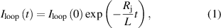
Figures 5(a)–(d) shows the angular dependence of I_cj and R_j at 4 K for 0.15, 0.20, 0.25, and 0.28 T, respectively. The vertical error bars for R_j, which are visible at 85° and 90° in figure 5(c), correspond to the standard uncertainty obtained from fitting. At 0.15 and 0.20 T, the measurements at high angles close to 90° were performed at intervals of 15° and 10°, respectively. This is because I_loop was expected to be considerably lower than I_cj, which caused negligible current decay.

Zoom In Zoom Out Reset image size

At a certain angle, I_cj decreased as the magnetic field increased. This was consistent with the field dependence of I_cj evaluated by transport measurements using a Bi-2223 superconducting joint sample [20]. The evaluated I_cj increased as the angle increased. The I_cj probably showed a broad peak at 90°, similar to the angular dependence of I_c for Bi-2223 tapes [1, 5].

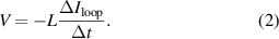
Figure 6 shows the smoothed V–I_loop curve at 0.15 T and 0–50°. We calculated the voltage from the I_loop–t curve at 300 s ⩽ t ⩽ 600 s using equation (2). When the decay of I_loop is significant, ΔI_loop becomes large and the calculated voltage is also large. The range of the calculated voltage varies with the angle. From the obtained V–I_loop curve, I_cj was evaluated at V_c of 10⁻⁸V for each angle. At 25–40°, I_cj was obtained from the intersection of V–I_loop and V_c, because V_c was within the voltage range of V–I_loop. At 0–20°, the V–I_loop curves were extrapolated using the power law (V = α I_loop ⁿ ) as shown by dashed lines in figure 6 because the voltage range was lower than V_c. I_cj was estimated from the intersection of the extrapolated V–I_loop and V_c.

Zoom In Zoom Out Reset image size

At 45° and 50°, the I_cj values estimated from the intersections were higher than the initially introduced I_loop of 220 A. Given that I_cj was estimated from the current decay, I_cj values higher than the initial I_loop value were not realistic. Thus, for 0.15 T, we employed I_cj only at 0–40°.

The I_cj values were evaluated in a similar way for 0.20, 0.25, and 0.28 T. I_cj values lower than the initial I_loop value (220 A) are shown in figure 5. This is the reason why I_cj at higher angles are not plotted.

The angular dependence of R_j with sample rotation can be divided into three regions: (i) low-resistance region (R_j of less than 1.4 × 10⁻¹³ Ω), (ii) transition region (three orders of magnitude changes in R_j to its maximum, R_j ^max), and (iii) high-resistance region (R_j of 10⁻¹¹–10⁻¹⁰ Ω). The angular dependence of R_j in each region is discussed below.

• (i)  
  Low-resistance region

This region is observed at high angles for each magnetic field. Figure 4(b) shows that the decay of I_loop at 75–90° and 0.25 T, corresponding to this region, was small. Because I_loop is considerably lower than I_cj, low R_j is realized and the persistent current continues to flow, as described in the previous section.

At 0.25 T and 75°, R_j was evaluated to be 1.4 × 10⁻¹³ Ω. The coefficient of determination (r²) in the fitting using the least squares method was 0.99. This implies that R_j can be obtained quantitatively. However, r² decreased at higher angles of 80–90° for 0.25 T, at which the lower R_j values were observed. As shown in figure 4(b), the I_loop–t curves were nearly flat at these angles. Although not visible in figure 3, the noise of V_Hall of ±5 × 10⁻⁷V influenced the I_loop–t curves, corresponding to ±2 ppm deviation in I_loop. Consequently, the uncertainty in the fitting for R_j derivation was large.

In region (i), for R_j of less than 4 × 10⁻¹⁴ Ω, r² was less than 0.8. This indicates that such low R_j values could not be quantitatively evaluated. Nevertheless, it is certain that the R_j values were less than the quantitative value of 1.4 × 10⁻¹³ Ω at 0.25 T and 75°. This indicates that the persistent current continued to flow in the sample owing to sufficiently low R_j.

• (ii)  
  Transition region

The value of R_j changed by approximately three orders of magnitude to its maximum (R_j ^max) in region (ii). Its values were evaluated quantitatively because r² was larger than 0.98 for each fitting.

As shown in figure 5, region (ii) shifted toward higher angles as the magnetic field increased. To clarify this shift, sections of R_j in region (ii) of figures 5(a)–(d) are shown in figure 7(a). Figure 7(b) shows this plot with the horizontal axis changed to B cosθ. The significant change in R_j at each magnetic field was nearly identical at B cosθ of 6–11 × 10⁻² T. The changes in R_j were independent of the magnitude of magnetic field.

Zoom In Zoom Out Reset image size

As described in the previous section, I_cj decreased owing to sample rotation with an increase in B_x = B cosθ. R_j is known to increase as the ratio of I_loop to I_cj increases, that is, as the load factor increases [30, 36, 38, 42]. In region (ii), the changes in R_j were due to the following reason. I_cj decreased as B_x = B cosθ increased owing to sample rotation. Because the change in I_loop by sample rotation is small, this decrease in I_cj caused an increase in the load factor. This resulted in a significant increase in R_j. The load factor values were not calculated, because I_cj could not be evaluated at most angles for each magnetic field in region (ii).

• (iii)  
  High-resistance region

This region eventually appeared when θ approached zero with sample rotation. High R_j values of 10⁻¹¹–10⁻¹⁰ Ω corresponded to the decay of I_loop by several amperes, as shown in figure 4(a).

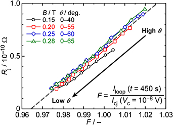
In region (iii), r² in the fitting ranged from 0.99 to 1.00, indicating that the R_j values were valid with sufficient precision. As shown in figure 5, R_j was higher at higher angles in each magnetic field. Using the evaluated I_cj values in region (iii), we quantitatively discussed the relationship between the load factor (F) and R_j. The value of F was calculated using equation (3) as follows:

$$\begin{equation}F = \frac{{{I_{{\text{loop}}}}\left( {t = 450\,{\text{s}}} \right)}}{{{I_{{\text{cj}}}}\left( {{V_{\text{c}}} = {{10}^{ - 8}}\,{\text{V}}} \right)}},\,\end{equation} \tag{ 3 }$$

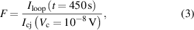
where t = 450 s corresponds to the median of the range of t used to obtain R_j (300 s ⩽ t ⩽ 600 s). The value of F can be larger than 1.00 when I_loop (t = 450 s) exceeds I_cj, because I_cj is determined by a considerably low voltage criterion, V_c = 10⁻⁸ V.

Figure 8 shows the relationship between F and R_j in region (iii), where the gray dashed line is derived using the least squares method. The value of F increased as the angle increased. The F values of 0.974–1.02 suggest that I_loop was comparable to I_cj. For F values of 0.974–1.02, R_j appeared to increase linearly. This suggests that, in region (iii), the change in R_j owing to sample rotation is primarily attributed to the change in F.

Zoom In Zoom Out Reset image size

When the sample is rotated, I_loop is probably influenced by the screening current and current sharing in the sample. The screening current is induced by sample rotation owing to an increase in B_x . Current sharing occurs when I_loop is close to or exceeds I_cj, typically in regions (ii) and (iii). However, as described in the previous section, the behavior of R_j could be explained using B cosθ and F in regions (ii) and (iii), respectively. This implies that the influences of the screening current and current sharing were sufficiently small in our measurements.

As explained in 3.2, we employed the I_cj values lower than the initially introduced I_loop of 220 A. Therefore, the highest angle at which I_cj was obtained was 65° at 0.25 and 0.28 T. If a larger I_loop is introduced, larger I_cj values can be evaluated at high angles near 90°.

In a preliminary measurement at 0.3 T, an introduced I_loop of 220 A decayed even at 90°. A persistent current of 220 A did not flow at 0.3 T. This means that region (i) was not observed at 0.3 T. To investigate the resistance transition from regions (i)–(iii) in this study, we chose 0.28 T as the maximum magnetic field.

At present, I_cj (I_c of the Bi-2223 superconducting joint) is lower than I_c of a tape [2, 4]. To ensure sufficient current margin, superconducting joints must be placed in a space at a low magnetic field in a magnet. In the 1.3 GHz (30.5 T) NMR magnet being developed, the magnetic field applied to the Bi-2223 superconducting joints is designed to be lower than 1 T [11, 25]. We believe that the magnetic fields of 0.15–0.28 T used in this study are in a realistic range for practical applications.

The angular dependence of R_j suggests that, in the design of a persistent-mode magnet, we must consider not only the magnitude but also the direction of a magnetic field applied to superconducting joints. The magnet must be designed such that superconducting joints are used in region (i). This allows for persistent-mode operation with a low R_j. If superconducting joints must be used in regions (ii) or (iii), additional efforts must be made to achieve a lower R_j. A recent study has shown that when I_loop is close to I_cj, R_j is almost inversely proportional to the elapsed time and decreases with an increase in the pinning potential of a superconducting joint [49]. This may be effective for achieving a lower R_j.

In region (iii), R_j decreased as F decreased. The relationship between F and R_j shown in figure 8 implies that a low R_j, as observed in region (i), may be achieved at F of less than 0.964. Evaluating the trend of R_j in detail at F equal to approximately 0.964 will help clarify the conditions under which a sufficiently low R_j for a persistent-mode operation can be achieved.