
Abstract
Magnetic switches apply AC magnetic fields to DC current-carrying high temperature superconducting (HTS) tapes to generate DC voltages and are commonly used in the persistent current switches (PCSs) and flux pumps to charge HTS-coated conductor magnets. Normally, they are made of copper field coils and iron cores with narrow air gaps for the HTS tape to pass through. However, the perpendicular components of the self-field of the HTS tape in the air gap can be enhanced by the iron cores and cause a critical current reduction of up to 40% to the tape. If ignored, this reduction, rather than the magnets themselves, will limit the current carrying capability of the HTS magnets. To tackle this problem, we present analytical approximations to calculate the self-field distribution of a superconducting tape between iron cores. The approximate solutions are based on the method of images in electromagnetics to simplify the derivation and are then verified by the experiments and 3D finite element method models using the T–A formulation. The solutions are universal and can be applied to almost all the magnetic switches currently in use. A case study of typical magnetic switches shows that the solutions can be used to determine the critical current reduction quickly and accurately, analyse the influence of different parameters, and simplify the design process of magnetic switches. The results can significantly benefit the design and optimisation of PCSs and flux pumps for HTS magnet charging systems in the future.
Export citation and abstract BibTeX RIS

Original content from this work may be used under the terms of the Creative Commons Attribution 4.0 license. Any further distribution of this work must maintain attribution to the author(s) and the title of the work, journal citation and DOI.
1. Introduction
With various promising applications in industry, research, and healthcare [1–5], high temperature superconducting (HTS) magnets are widely considered a superior substitute for conventional copper wire magnets and permanent magnets towards devices with smaller volumes and lower losses [6]. HTS magnets can be made closed-loop and independent of power sources thanks to the zero resistivity and thus the persistent current in the superconductors [7]. After cooling the system and charging the closed-loop magnets, a power-source-free and even a cooling-source-free magnet system can be realised if the operation time of the devices is not too long [8]. However, as the precondition of realising this, a closed-loop HTS magnet needs to be adequately charged. So far the proposed charging methods can be roughly classified into two types, persistent current switches (PCSs) [9] and flux pumps [10]. The basic ideas of the two methods are the same: to generate a voltage high enough to inject current into the superconducting loop. External conditions can be applied to part of the HTS loop to generate the voltage, such as heat [11], overcurrent [12], and magnetic field [13]. Recently, magnetic field-controlled PCSs and flux pumps [14] are popular because no bulky power sources or leads are required and the voltage can be generated by the 'dynamic resistance' [15] without driving the superconductor normal.
When a DC current-carrying HTS tape is exposed to AC magnetic fields, a DC voltage positively related to the magnetic field can be measured [16], which can be used to charge the magnets. The ratio of this voltage and the DC current is the so-called 'dynamic resistance'. To apply an AC magnetic field high enough, magnetic switches (copper-wired electric magnets with iron cores) are normally used [17]. Figure 1(a) shows the two typical magnetic switch designs in PCSs and flux pumps. The tape can pass through the iron cores transversely (Case I: the open-loop case) and longitudinally (Case II: the closed-loop case). These switches are designed to maximise the voltage generated by the dynamic resistance, which is the key parameter in magnetic field-controlled PCSs and flux pumps. Previous work has shown that the dynamic voltage is proportional to the length of the tape exposed to the AC field [18]. In the open-loop case in figure 1(a), the tape can loop through the gap back and forth for several times to extend the contact length, which is suitable for large-scale magnets that require large charging voltage. The closed-loop case only allows the tape to go through once if the other gap is not available (e.g. a round core with a slit) so it works well for small magnets due to the simplicity.
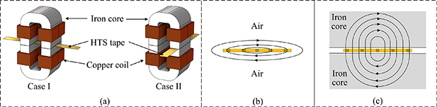
Figure 1. (a) Two typical magnetic switch designs used in PCSs and flux pumps. (b) and (c) The magnetic field distribution of a current-carrying HTS tape (cross-section) in the air and between the iron cores.
Download figure:
Standard image High-resolution imageWhen the magnet is fully charged and the switch stops working, the self-field of the tape between the iron cores will be significantly changed due to the high permeability of the iron. As shown in figures 1(b) and (c), influenced by the iron core, this self-field will be mostly perpendicular to the tape, and thus a critical current (Ic) reduction will happen due to the field dependency of the normal undoped HTS tapes. Since the Ic is very sensitive to the perpendicular field, this reduction can be considerable, which will be shown in detail in this paper. The situation can be even worse when charging large-scale HTS magnets with a high inductance and many joints. To increase the charging voltage, the air gap for the tape passing through is very narrow, the permeability of the iron is very high, and many switches are used on one tape [19]. Without considering this Ic reduction, the Ic of the magnet would be limited by the switches rather than the magnet itself. Hence, it is essential to calculate the self-field distribution of a superconducting tape passing through a narrow gap between iron cores, according to which the Ic reduction can be then determined.
In this paper, we present analytical approximations to the self-field distribution of a superconducting tape carrying a DC current between iron cores. The derivation of the approximate solutions is based on the method of images in electromagnetics. Iron cores with and without a closed magnetic circuit are discussed and the results can be applied to almost all the magnetic switches. Based on reasonable assumptions, a simplified solution is obtained, with which the Ic reduction can be obtained fast and easily. To verify the analytical solution and apply it to practical application, a case study of two typical magnetic switches is considered. The Ic reduction is measured experimentally and calculated analytically, and a 3D finite element method (FEM) simulation model is built. The results obtained through three methods can validate one another and provide different insights into understanding this problem. With the verified analytical approximations, influences of different parameters of the switches on the critical current are discussed.
2. Problem definition and simplification
To determine the Ic reduction of the superconducting tape between the iron cores, the primary problem is to calculate the magnetic field distribution on the surface of the tape. Combining this with the field dependent Ic curve provided by the HTS tape manufacturer, the Ic reduction can be easily figured out. In this paper, we define two typical cases for calculation, which we believe can cover most of the magnetic switches geometrically.
To abstract a mathematical model for calculation from the practical problem, some necessary assumptions must be made. Compared with the real magnetic switch, the assumptions and idealisations used in this paper include:
- (a)Instead of a 3D problem, a 2D infinite long model is considered, which can be regarded as the cross-sectional area perpendicular to the tape length direction.
- (b)Since the width to thickness ratio of HTS tapes is extremely large, usually between 1000 and 10 000 [20], the thickness of the tape is neglected here, which means the tape can be represented by a straight line of a certain width with a current line density J flowing inwards or outwards the plane.
- (c)The iron cores are regarded as infinite above or beneath the boundary with the air gap. The width of the iron cores is also infinite because the real width of the iron core is usually much greater than the air gap length g.
- (d)A constant permeability μ1 is applied to the iron rather than a B–H curve to simplify the calculation. The magnetic field generated by a single tape is still far away from the saturation point of the iron, which means the iron mostly works in the linear region of the B–H curve.
- (e)The current distribution inside the tape is homogeneous. This assumption is only sensible when the current is close to the critical current because otherwise, the current would concentrate on the edge areas while the middle part of the tape is almost current-free. This study focuses on the critical state of the tape, which justifies this assumption.
With the assumptions above, the two mathematical cases to solve are shown in figure 2. In case I, the geometry is symmetric and can represent those magnetic switches without closed magnetic circuits. In case II, the two half-infinite planes connect each other at infinity, which can represent switches with closed magnetic circuits around the current density J, i.e. the field source. We call case I and II the 'open-loop case' and 'closed-loop case', respectively. The problem to solve in this paper is the perpendicular field distribution along the tape width direction when there is a certain DC current density flowing in the tape.

Figure 2. The two mathematical models to solve. In case I, an infinite plane filled with iron is divided into two half-infinite planes by an air gap, which represents the magnetic switches without closed magnetic circuits; in case II, the two half-infinite planes are connected somewhere at infinity, which represents the switches with closed magnetic circuits. J is the current line density in the tape; g is the air gap length; μ0 and μ1 are the permeability of the vacuum and the iron core, respectively.
Download figure:
Standard image High-resolution image3. Analytical approximations
Figure 2 shows a magnetic field distribution problem with certain conditions. If we define A as the magnetic vector potential, it satisfies

where B is the magnetic flux density. The Poisson's equation governing the air gap is

The Laplace's equation governing the iron cores is

On the two boundaries, the boundary conditions of B and the magnetic field H are
and
where B 0, B 1, B 2, H 0, H 1, H 2 are the magnetic flux density and magnetic field strength of the air gap, iron of the upper plane, and iron of the lower plane, respectively. n 01 and n 02 are the normal vectors of the two boundaries.
By combining equations (2)–(5), the problem can be solved. Normally, they are solved numerically by FEM using commercial software, because it is rather difficult to derive an analytical solution out of them. However, with this geometry shown in figure 2, an accurate solution is not impossible using the method of images.
3.1. Method of images
The method of images is a standard method in electromagnetics to calculate the field without solving the Poisson's or Laplace's equations. It is based on the uniqueness theorem of the Poisson's equation [21]. We only give the conclusions, which will be used in this paper. More details about this method can be found in [22].
As shown in figure 3(a), the lower and upper half-planes are filled with media having a permeability of μ0 and μ1, and there is an arbitrary current density J in the medium μ0. To calculate the magnetic field distribution in the medium μ0, the method of images can be used. As shown in figure 3(b), the entire plane is now filled with medium μ0. Compared with (a), the Poisson's equation in the lower half-plane is the same. To maintain the boundary conditions of B and H unchanged, an image current density J' is placed in the upper half-plane at the same distance to the boundary as the source current density J. And J' should satisfy

Figure 3. A schematic for the method of images.
Download figure:
Standard image High-resolution imageNow, with the same Poisson's equation and boundary conditions, the field distributions in the lower half-plane for the two cases in figure 3 are the same. The distribution of B or H in (b) can be easily calculated using the Biot-Savart law since it is the superposition of the fields generated by the image and source current density.
3.2. Approximate solutions for case I
In the open-loop case, there are two media μ0 and μ1, and two parallel boundaries. According to the method of images, the HTS tape J should have two images to the two boundaries, J1 and J2, and
One should note that the image current density J1 and J2 should also have images J3 and J4. By repeating this process, a series of an infinite number of images is obtained as shown in figure 4. The values of these image current densities are
Now the problem has been converted into calculating the self-field of a tape stack containing an infinite number of tapes. A Cartesian coordinate system is chosen as shown in figure 5. The tape width is 2a. The magnetic field H at point P (x, y) is the superposition of the field generated by the source current J and all the image current density Jn. According to the Ampere's law (or the Biot-savart law), the y component of the magnetic field strength H generated by the element (η) is
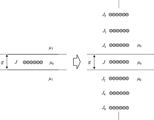
Figure 4. Applying the method of images to the open-loop case.
Download figure:
Standard image High-resolution image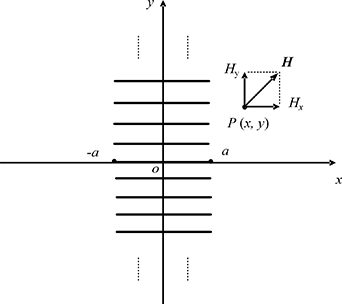
Figure 5. Coordinate system and the parameters used to calculate the field distribution of the infinite tape stack.
Download figure:
Standard image High-resolution imageTherefore, the y component of the field at P (x, y) generated by the source tape (from -a to a) is
One should note that in the two equations above, J is the current line density, and
where I is the DC current in the HTS tape. Using equations (8) and (10), the y component of the self-field of the infinite tape stack can be obtained by superposing all the currents
where N is an integer. One should note that equation (12) can only be used to calculate the field distribution in the air gap, but not in the iron core. In a similar way, the x component Hx can be calculated. However, since Hy is dominant in the air gap and the impact of the parallel field on the HTS tape is small [23], Hx is ignored in this paper.
3.3. Simplified analytical solutions
Equation (12) shows that Hy is a 2D infinite series function dependent on several parameters, I, a, μ, μ0, and g. It is straightforward to use software (e.g. MATLAB) to calculate the exact value of this solution by assigning N a rather great value (e.g. 10 000). However, it is possible to further simplify this solution if more assumptions are taken.
In practice, the permeability of the iron μ1 is usually much greater than that of the vacuum μ0, which means equation (8) can be approximated as

And for an infinite tape stack, the thickness is infinite, which is much greater than the width of the stack, 2a. Therefore, as shown in figure 6, the self-field of such a stack can be approximated as the self-field of a line current with an infinite length in the y-direction and zero-width in the x-direction. The field distribution of such an infinite line current can be easily calculated using Ampere's law. The magnetic flux density on the left and right half-planes are in the opposite directions and of the same value, which is
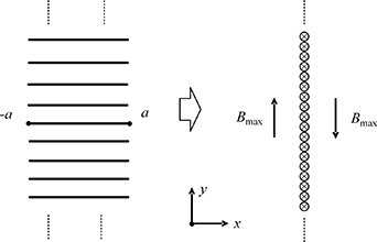
Figure 6. Approximation for a simplified analytical solution for the open-loop case.
Download figure:
Standard image High-resolution imageEquation (14) is much simpler than (12), but it can be only used to calculate the field distribution when |x| ⩾ a since the width of the tape stack is ignored. The problem we are solving is to calculate the field on the surface of the tape, which means that equation (14) is useful to obtain the flux density on the left and right edges of the tape where |x| = a. When |x| < a, the flux density should be smaller than that on the edges, so we name the flux density Bmax in equation (14). With this maximum value known, the field distribution from -a to a can be fully obtained if we know the field changing trend when |x| < a.
For the infinite stack in figure 5, we have the Ampere's law
where Js is the average current density of the stack and
Here we have taken a further assumption that the current density is also homogeneous along the y-direction, which is sensible because the gap length g is usually much smaller than the tape width 2a. Now, the model resembles the 'infinite slab' in the Bean model [24]. When B is homogeneous along the y-direction in this infinite tape stack, equation (15) becomes
This means that By changes linearly along the x-direction with a constant slope. Given that it is obvious that By is 0 at x = 0, the perpendicular field distribution on the tape surface can be obtained as
where |x| < a. This result agrees with equation (14) at |x| = a.
3.4. Approximate solutions for case II
In the closed-loop case, the iron is connected at infinity, which means there is a second magnetic circuit in addition to the one through the air gap. As shown in figure 7, the two magnetic circuits are parallel and thus independent of each other. Therefore, the magnetic field in the air gap should be the superposition of the field calculated from these two magnetic circuits.
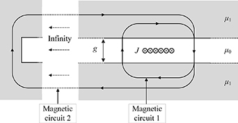
Figure 7. The two magnetic circuits in the closed-loop case.
Download figure:
Standard image High-resolution imageSince magnetic circuit 1 is the same as the open-loop case, the analytical solution to the open-loop case can be used directly. According to the simplified solution, the perpendicular magnetic flux density on the tape surface should be a straight line along the x-direction as shown in figure 8. The maximum value B1 can be known from equation (18) as

Figure 8. Superposition of the two magnetic circuits.
Download figure:
Standard image High-resolution imageSuperposed by magnetic circuit 2, the field of the closed-loop case should be of the same profile as the open-loop case, but with a DC offset B2, which can be calculated from magnetic circuit 2. If we introduce an unknown k to describe the length ratio of the tape where the magnetic flux density is positive, an equation can be obtained from the similar triangles in figure 8.
which can be simplified as
One should note that the magnetomotive force (MMF) of magnetic circuit 2 is kI rather than I. According to the Ohm's law in magnetic circuits, we have
where Rm is the magnetic resistance at infinity. In normal cases, μ1 is much greater than μ0. If we assume at infinity there is an air gap with a length of g' (which is not shown in figure 7), the equation can be approximated as
Combing equations (19) and (23), we have
Solving simultaneous equations (21) and (24), B2 and k can be calculated as
Now we can conclude that the field distribution along the tape width direction for closed-loop switches is a straight line from B1–B2 to -B1–B2, with B1 and B2 both known.
4. Case study—magnetic switches in flux pumps
After deriving the analytical approximations for both cases in figure 2, the solutions will be used to solve a practice case of a typical magnetic switch used in a transformer-rectifier flux pump. The critical current reduction due to the iron core will be determined analytically, experimentally, and numerically, from which the validity of the analytical solutions will be verified. The impact of the switch parameters on the switch performances will also be discussed.
4.1. Case description
The two cases in figure 1(a) are different in terms of the self-field distribution discussed in this paper. For the open-loop case, the iron core and the tape along the tape width direction are symmetric, which fits the model of the open-loop case in figure 2; for the closed-loop case, the distribution is asymmetric, because there is an additional magnetic circuit in the iron core allowing the magnetic flux to form a closed loop around the tape, which fits the model of the closed-loop case in figure 2. The parameters of the switches are shown in table 1. When the charging process is completed, there is no current in the copper coils of the magnetic switches and a DC current has been injected in the tape as part of the HTS magnet. With the analytical approximations, the perpendicular field distribution on the tape surface can be calculated. With the calculation result and the Ic-perpendicular field curve obtained from the HTS tape manufacturer, the Ic reduction can be determined.
Table 1. Parameters of the magnetic switches.
| Parameters | Value | |
|---|---|---|
| Iron core | Model | AMCC-40 |
| Permeability (linear region) | 12.72 × 10⁻³ H m−1 | |
| Mean magnetic pass length | 194 mm | |
| Effective length | 35 mm | |
| Effective width | 13 mm | |
| HTS tape | Manufacturer | American Superconductor (AMSC) |
| Tape thickness | 0.2 mm | |
| HTS layer thickness | ∼1 μm | |
| Tape width | 12 mm | |
| HTS layer width | 10 mm | |
| Critical current (77 K, s.f.) | 248 A | |
| n-value | 35 | |
aThe length and width of the effective cross-section area of the magnetic pass.
4.2. Solution verification
To verify the analytical solution, a full-scale 3D FEM model is built in COMSOL Multiphysics. This model uses the T–A formulation [25] to introduce the non-linear E–J relationship (27) into equations (1)–(5). In the T–A formulation, the current vector potential T is used to calculate the current density J , and the magnetic vector potential A is used to calculate the magnetic flux density B . The E–J relationship is
where E0 = 1 × 10⁻⁴ V m−1. ρ is the resistivity of the superconductor. The value of n can be found in table 1. Jc(B) is the perpendicular field-dependent critical current density and is obtained from AMSC. It should be noted that the AMSC HTS tapes used in this paper is undoped and the critical current is maximumly reduced when the external field is perpendicular to the ab plane of the tape. The parallel field dependency is ignored in this paper [23]. In this model, the thickness of the HTS layer is ignored [25]. Rather than the constant permeability, the B–H curve of the iron core is used for an accurate result. The HTS tape length in the model is 10 cm, which makes the quench voltage criterion 10 μV. The voltage is calculated in the model by the integral
where S is the total area of the tape, and w_tape is the HTS layer width (10 mm). The tape length is in the z-direction. The air gap length g is set as 0.2 mm, the same as the tape thickness, which means there is no extra space between the tape and the iron core.
According to the simulation results, when the DC currents in the tape are 160 A for the open-loop case and 150 A for the closed-loop case, V_tape reaches the quench voltage criterion criterion of 10 μV. If we input the corresponding parameters into the analytical solution (12), the distribution of By long the x-direction can be obtained. For the open-loop case, the comparison of the analytical and simulation results is shown in figure 9. When calculating equation (12), the integer N must be a certain value instead of infinity. Therefore, the results of different N are given in the figure. As N becomes larger, the curve is closer to the simulation result. The fact that curves for N= 1001 and N= 10 001 are almost overlapped indicates that the tapes from the 1000th away in the infinite tape stack hardly influences the field distribution around the source tape. The analytical solution shows the field curve is linear along the x-direction, which agrees with the simplified solution (18). However, the simulation result shows that the curve is not completely linear. This difference is caused by the assumption that the current density is homogeneous along the x-direction, which does not completely represent the real case. Besides this, the analytical results and the simulation show good consistency. As shown in figure 9. The maximum value of By is around 0.5 T. This value can also be calculated from the simplified solution (18) as 0.503 T.
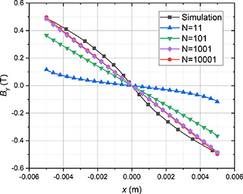
Figure 9. Comparison of the analytical and simulation results on By distribution along the x-direction in the open-loop case. I = 160 A; g = 0.2 mm.
Download figure:
Standard image High-resolution imageFor the closed-loop case, there is an identical air gap in the left part of the iron core, which means g' = g in equations (25) and (26). Then we have
where B1 = 0.47 T, which can be obtained from the open-loop case when the current is 150 A. The solution is a straight line from B1-B2 (0.31 T) to -B1-B2 (0.63 T). The comparison of the analytical and simulation results is shown in figure 10. The tape length ratio k can be seen as 1/3 from the figure, and again, a good consistency can be observed.

Figure 10. Comparison of the analytical and simulation results on By distribution along the x-direction in the closed-loop case. I = 150 A; g = 0.2 mm.
Download figure:
Standard image High-resolution image4.3. Critical current reduction
Now, with the analytical approximations for both cases in figure 1(a), we can determine the critical current reduction of the HTS tape based on the given conditions. If the air gap length is fixed, for any given current value I, the perpendicular field distribution along the tape width can be calculated. Since the field is nearly linearly distributed, the average field can be easily obtained. Then, with this average perpendicular field, a corresponding critical current can be found from the Jc(B) curve provided by the tape manufacturer. Therefore, the critical current of the tape is dependent on the current flowing inside it and can be seen as a function of the current Ic (I).
Figure 11 shows the function Ic (I) for both cases in figure 1(a). To find the degraded critical current of the tape, we need to find the point where


Figure 11. The critical current as a function of the tape current. The air gap is 0.2 mm long.
Download figure:
Standard image High-resolution imagewhich is also shown in figure 11. For the open-loop case, the degraded critical current is 159 A, which means within this point, the critical current is larger than the current and the tape is in the 'safe region'; beyond this point, the critical current would be lower than the current, and the tape quenches. This result also agrees with the simulation results above, which indicate a current 160 A when the voltage reaches the quench criterion of 1 × 10⁻⁴ V m−1.
For the closed-loop case, the critical current is 153 A, slightly smaller than that of the open-loop case. The small difference seems unreasonable because the DC offset B2 in the open-loop case is 1/3 of B2. But if we calculate the average absolute value of the perpendicular magnetic flux density for the two cases, we have
where k = 1/3. So
which indicates that the impact of k is quite small on the average perpendicular field to the tape. This justifies the small critical current difference between the two cases.
To verify the results above, we measured the critical currents of the taps in the two switches in figure 1(a). The distance between the two voltage taps is 10 cm. The results are shown in figure 12. The critical current for the open-loop case is measured as 136 A, and that for the closed-loop case is slightly smaller. The self-field critical current of the tape is measured as 248 A, and that for a half iron core is slightly smaller. This means if the magnetic circuit is not closed, it could barely influence the critical current of the tape. The experimental results (136 A) show there is an error of around 17% for the analytical solution (159 A) and the 3D FEM model (160 A). This error suggests that the practical current reduction is even worse than that seen in the analytical approximations. This is sensible because, except for the experimental errors and the assumptions we take to simplify the problem, the analytical approximations only consider the electromagnetic aspect of the problem. There are other factors that impact the HTS tape performance, e.g. mechanical factors. For instance, according to the analytical and simulation results, when the current is around 160 A in the tape, the maximum magnetic flux density on the tape surface is around 0.5 T. There is a large attractive force between the two iron cores, which is applied to the tape in the middle. The impact of this force on the tape performance is not considered in the analytical approximations and the simulation model. Therefore, the current reduction suggested by the analytical approximations in this paper is only a lower limit, while the practical reduction is usually worse.
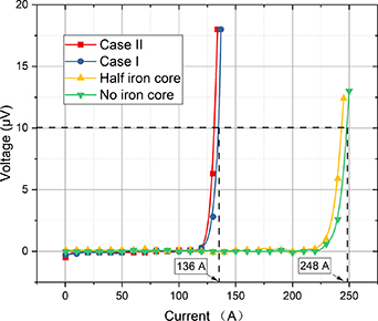
Figure 12. Measured critical currents with and without the iron cores at 77 K. 'Half iron core' means the upper half of the iron core is removed. The air gap is 0.2 mm long.
Download figure:
Standard image High-resolution image4.4. Influences of contact length of the iron core and the tape
The magnetic switches are supposed to generate voltage high enough to charge the magnet when used in a flux pump. Previous studies [17] show that the voltage is proportional to the exposed length of the tape where the AC field is applied, which is the contact length of the iron core and the tape in figure 1(a). From the simulation results obtained from the 3D model, figure 13, we can also see the current density distribution is rather homogeneous along the tape length direction, which means the voltage generated by the tape per unit length should be equal. The current density ratio J/Jc(B) of the tape contacting the iron core is higher than 1 because this part of the tape needs to generate a voltage high enough to reach the quench criterion of 10 µV for the entire tape length (10 cm) while the rest of the tape generates almost zero voltage with a ratio below 0.8.

Figure 13. Simulation results of J/Jc(B) of the HTS tapes in the open- and closed-loop cases. The colour shows the ratio, and the arrows show the magnetic flux flow. I = 160 A in the open-loop case; I = 150 A in the closed-loop case; g = 0.2 mm.
Download figure:
Standard image High-resolution imageHowever, since the analytical approximations are based on a 2D infinite long model, it seems impossible to investigate the impact of this contact length on the critical current reduction. Therefore, the contact lengths are changed in the 3D FEM model of the closed-loop case, and the results are shown in and table 2.
Table 2. Critical currents for different contact lengths.
| Contact length (mm) | Critical current (A) |
|---|---|
| 8.75 | 153 |
| 17.5 | 152 |
| 35 | 150 |
From the table we can tell the critical current is not sensitive to the change in the contact length. The original length of the iron core is 35 mm, and with the length reduced by half twice, the critical current only increases by 2 A and 1 A. The reason for this lies in the non-linear E–J characteristic of the HTS tape (27). When the length is reduced from 35 mm to 17.5 mm, if the current is maintained at 150 A, the voltage would decrease from 10 µV to 5 µV. To compensate for this 5 µV difference, the current must increase. However, the tape is already working at the steep region of the E–J power curve, which means even if the current increases slightly, the voltage will increase sharply. Therefore, as shown in table 2, the 2 A current will generate this 5 µV to make the total voltage back to the criterion of 10 µV. Thanks to this insensitivity of the critical current reduction to the contact length, the 2D analytical approximations are still able to give a good estimation for magnetic switches with different contact lengths.
4.5. Influences of air gap length
According to the magnetic circuit law, if the MMF of the copper coils of a magnetic switch is fixed, the magnetic flux density in the air gap is approximately inversely proportional to the air gap length. Therefore, a small g means that the effective AC field applied to the tape can be increased, which can be used to generate a high voltage to charge the magnet. However, the analytical approximations also show that a small air gap length can cause a large critical current reduction. Using the method shown in figure 11, we have calculated the critical currents for different air gap lengths, and the results are shown in figure 14. The reduction for a g smaller than 0.5 mm can be over 30%, which must be considered in the design process of the PCSs or the flux pumps. When the air gap length is larger than 1 mm, the reduction is only less than 10%. Hence, we recommend the air gap length in a magnetic switch should be larger than 1 mm to mitigate the reduction, given that it is very unlikely the critical current of a magnet can reach 90% of the tape critical current.

Figure 14. The impact of the air gap length on the critical current of the tape.
Download figure:
Standard image High-resolution image
5. Conclusion
In this paper, we derived the analytical approximations for the perpendicular self-field of a superconducting tape between the two iron cores. A 2D infinite long mathematical model is abstracted, in which the problem is divided into two cases, a symmetrical one and an asymmetrical one with an additional magnetic circuit. For the open-loop case, instead of solving the Poisson's equation, we use the method of images to simplify the derivation, with which the mathematical model is converted into an infinitely thick tape stack. The solution of the self-field distribution of the stack is obtained as an infinite series, shown as equation (12). To simplify the solution, more assumptions are taken and the simplified solution is obtained as equation (18). Then, the closed-loop case is solved using the conclusion from the open-loop case and the magnetic circuit law. The results are equations (24)–(26).
To verify the analytical approximations and demonstrate their application, we give a case study on two typical magnetic switches. The critical currents of the two cases are measured to determine the critical current reduction experimentally; a 3D FEM model using the T–A formulation is built to verify the field distribution. The experiment proves the large critical current reduction predicted by the approximations, and the simulation results agree well with the analytical approximations. The influences of the air gap length and the contact length of the tape and the iron core are then analysed. Important conclusions are obtained, e.g. the critical current is not sensitive to the contact length, and the air gap length is recommended as 1 mm or larger.
The analytical approximations derived in this paper are universal and can be applied to most magnetic switches with different parameters. The approximations can help us better understand the physical mechanism, and the results indicate the critical current reduction caused by the self-field can be considerable. One should take this reduction into consideration when designing a charging system of HTS magnets, and the analytical approximations presented in this paper can make this process fast and easy.
Data availability statement
All data that support the findings of this study are included within the article (and any supplementary files).