
Abstract
In recent years, the T-A formulation has emerged as an efficient approach for modelling the electromagnetic behaviour of high-temperature superconductor (HTS) tapes in the form of coated conductors (CCs). HTS CCs are characterized by an extremely large width-to-thickness ratio of the superconducting layer, normally up to 1000 ∼ 6000, which in general leads to a very large number of degrees of freedom. The T-A formulation considers the superconducting layer to be infinitely thin. The magnetic vector potential A is used to calculate the magnetic field distribution in all simulated domains. The current vector potential T is used to calculate the current density in the superconducting layer, which is a material simulated with a highly nonlinear power-law resistivity. This article presents a review of the T-A formulation. First, the governing equations are described in detail for different cases (2D and 3D, cartesian and cylindrical coordinates). Then, the literature on the implementation of T-A formulation for simulating applications ranging from simple tape assemblies to high field magnets is reviewed. Advantages and disadvantages of this approach are also discussed.
Export citation and abstract BibTeX RIS

Original content from this work may be used under the terms of the Creative Commons Attribution 4.0 license. Any further distribution of this work must maintain attribution to the author(s) and the title of the work, journal citation and DOI.
1. Introduction
The availability of high temperature superconductors (HTS) at lengths over a kilometre has enabled the development of several applications, some of which have already reached a pre-commercial stage. For the design of HTS applications, numerical modelling plays a key role, especially when the electromagnetic behaviour needs to be investigated. Here, the electromagnetic characterisation of superconductors in general and HTS in particular is quite peculiar, due to the anisotropic critical current density in HTS materials. In addition, the numerical methods adopted for conventional materials are often not applicable.
Over the years, different approaches to model the macroscopic electromagnetic behaviour of HTS have been proposed [1]. Among them, the H formulation became the most widely used method in the applied superconductivity community [2, 3], although other methods, such as the minimum electro-magnetic entropy production method [4], proved to be more efficient from the computational point of view [5]. The main reason for the success of the H formulation is its ease of implementation in the widespread commercial software package COMSOL Multiphysics. This enabled researchers who are not necessarily experts in the field to use numerical modelling and made it easy for research groups as well as the whole community to share finite element method (FEM) models and transfer knowledge.
One of the limitations of the H formulation is its computational speed in cases that contain large numbers of superconducting tapes (or coil turns), especially in the case of HTS coated conductors: those superconductors are characterized by an extremely large width-to-thickness ratio of the superconducting layer, which leads to a considerable increase of the total number of the degrees of freedom (DOF) of the problem.
In recent years, the T-A formulation has proved to be a competitive alternative for modelling systems with a large number of HTS coated conductors, where the superconducting layer is regarded as an infinitely thin sheet and the variation of the electromagnetic quantities across its thickness can be neglected [6, 7].
This article provides a review of the works based on the T-A formulation and is organized as follows. Section 2 describes the governing equations of the formulation in 2D and 3D, including the extension to the homogenisation and multi-scale approaches, used to handle cases with large numbers of HTS tapes. The validation of the methodology as well as an efficiency analysis is reported in section 3. Section 4 is dedicated to applications: it starts with basic tape and coil modelling, then addresses several power applications, and it finally concludes with high field magnets. Section 5 contains a discussion on the T-A formulation, highlighting its advantages and disadvantages. Eventually, section 6 draws the main conclusions.
2. T-A formulation
The T-A formulation was first introduced by Zhang et al [6] and Liang et al [7] in 2016. The concept of this numerical model is to solve the current vector potential T only in the superconducting domain, while the magnetic vector potential A is solved for the whole domain. The two state variables T and A are used to calculate the current density J and the magnetic flux density B , respectively. The numerical model is fully coupled by solving for both J and B at the same time and continuously exchanging these variables.
2.1. General formulation
The governing equations of the general form are,


The resistivity in type II superconductors is modelled by the E-J power law, coupling the local electric field with the local current density within the superconducting domain only

Here, ρHTS denotes the resistivity of the HTS material, Jc is the critical electric field at 10−4 V m−1, Jc is the critical current density and n is the superconducting n-value. Both Jc and n can depend on the magnetic field.
Applying Maxwell-Faraday's law to the HTS domain gives
In the whole domain Maxwell-Ampere's law is applied to solve the traditional A formulation

where μ0 and μr are the magnetic and relative permeability of the free space, respectively.
The current density is coupled with the A formulation by an applied external surface current density J e

where δ denotes the thickness of the HTS tape. J e is imposed in the tape in A m−1 to accommodate for the thin strip approximation, which is neglecting the thickness of the HTS layer.
The transport current flowing in the superconductor is applied at the tape terminals. It can be represented by an integral of the current density over the cross-section of the conductor
Here, S is the cross section of the conductor and ∂S represents the boundary edges of the cross section.
2.2. Formulation in 2D (infinitely long strip, axial-symmetric)
Due to the high aspect ratio of HTS coated conductors, modelling the whole surface requires long simulation time. The T-A formulation makes unique use of this issue, by applying the thin strip approximation to the tape. This geometrical simplification reduces the surface area of the HTS tape to a thin sheet (figure 1).

Figure 1. T is computed only in the superconducting domain (black lines), while A is computed everywhere. The thickness of the HTS tape is collapsed into a superconducting layer, represented by a 1D line element. The current is enforced by boundary conditions at the edges T1 and T2 of the tape.
Download figure:
Standard image High-resolution imageTherefore, the current is restricted to flow within the superconducting sheet, while
T
is reduced to the component perpendicular to the tape. The current vector potential can then be defined as  , where
 ![${\boldsymbol{{n}}} = {\left[ {\begin{array}{*{20}{c}} {{n_x}}&{{n_y}}&{{n_z}} \end{array}} \right]^T}$](https://content.cld.iop.org/journals/0953-2048/35/4/043003/revision2/sustac5163ieqn2.gif) and
and  are the normal vectors perpendicular to the wide face of the superconducting tape in cartesian and cylindrical coordinates, respectively. In 2D the surface element of the HTS tape is reduced to a 1D line element and equation (1) can be written as
in cartesian coordinates, or for axial-symmetric problems in cylindrical coordinates as
Depending on the orientation of the tape,  or
or  in equation (8) can further be neglected. Equation (9) expresses a general case for a tape wound with an 'easy bend' where the current flows in the
  direction, which reduces the current vector potential to
  . Furthermore, when implementing Faraday's law, equation (4) can be reduced to
for cartesian and cylindrical coordinates respectively. Again, only the x or y component of the magnetic flux density in cartesian coordinates needs to be considered, depending on the orientation of the tape.
A transport current, as defined in equation (7), can then be applied to the edges of the tape using

where T1 and T2 are the current vector potentials at the respective edge points and δ is the thickness of the superconducting tape.
2.3. Formulation in 3D
In a 3D geometry, the superconductor is no longer represented as a line, instead the conductor will be modelled as a thin sheet [6]. This surface element also does not consider the thickness of the HTS. Using the same set of equations for a 3D geometry, the current density vector is defined as
The implementation of Faraday's law in the superconducting domain can now be written as
The boundary condition for the transport current is applied in the same way as for a 2D problem in equation (12), only instead of defining it at the terminal points, it is applied to the edge of the superconducting sheet. In 3D there is an additional boundary condition to consider. When symmetry is exploited the conductor cross section is defined with a zero-flux condition in the T formulation to contribute with the magnetic insulation boundary condition of the A formulation.
2.4. Multi-scale and homogenisation method
Based on the general form of the T-A formulation, two simplification methods can be implemented in order to reduce the amount of computational resources needed to model large numbers of tapes in 2D and 3D. Although simplification assumptions are made, the accuracy for hysteresis losses, current distribution and magnetic field distribution is maintained [8]. Both these methods have been validated in 2D by [8, 9] and in 3D by [10, 11].
2.4.1. Multi-scale method.
In the multi-scale method, the current vector potential is defined for each analysed tape individually.
The current density distribution is obtained by computing T in the analysed tapes, while the non-analysed tapes in between are approximated by linear interpolation, shown in figure 2. The magnetic flux density is computed via the A formulation, which is defined in the whole space. In order to couple the T and A formulation, the current density is imposed into the A formulation using equation (6), where J is multiplied by the thickness of the tape, to obtain the surface current density.
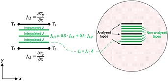
Figure 2. T-A multi-scale approach in 2D. In this example, there are three analysed tapes (black) whereby J is obtained by computing T. J in the remaining non-analysed tapes (green) is approximated by linear interpolation. The surface current J e is imposed in the A formulation by means of a boundary condition. See also [8].
Download figure:
Standard image High-resolution image2.4.2. Homogenisation method.
The homogenisation method assumes that a stack of tapes can be considered as an anisotropic bulk, which will not compromise the electrodynamic behaviour of the coil [8]. In the T-A formulation, a tape is considered as a thin sheet with the thickness δ, where we now define a unit cell around it with the thickness Λ. The unit cell assumes the thickness of the additional layers in a HTS tape such as copper, hastelloy, buffer layer, insulation material, but the materials themselves are not modelled separately. Therefore, the actual size of the bulk is given by the stack of tapes with the unit cells surrounding them. The tapes are then transformed into a single block, which is shown in figure 3.

Figure 3. T-A homogenisation in 2D. The superconducting sheets are replaced by a homogeneous bulk. The current density inside the bulk is computed by boundary conditions applied to the edges T 1 and T 2 of the bulk and the scaled current density J e is imposed in the A formulation.
Download figure:
Standard image High-resolution imageThe scaled external current density J e in the homogenized bulk is imposed in the A formulation using,
When expanding the homogenisation method to 3D geometries, software like COMSOL only features the normal vector on boundary elements. Therefore, it is necessary to define the normal vector  inside the bulk.
Considering a simple 3D geometry that is commonly studied like in the case of a racetrack coil,  will be defined for the straight and circular part respectively
Here,  defines the normal vector in a cartesian coordinate system and
  is defined in a cylindrical frame.
The boundary conditions for the transport current are applied in the same way as in the 3D tape model, with Dirichlet boundary conditions at the top and bottom of the homogenized bulk. For the additional boundaries that come from the homogenisation technique, a Neumann boundary condition is defined as,

In a 2D homogenisation problem, equation (18) can be reduced to only the scalar component of T .
In the case of a closed coil, symmetry conditions can be useful to simplify the problem. When considering a quarter model, the symmetry planes use a zero flux condition for the superconducting domain. In the A formulation the symmetry plane is considered a perfect magnetic conductor, mirroring the current of the superconductor.
3. Validation of modelling strategies
The validation of the T-A formulation, especially of the advanced modelling strategies (multi-scale, homogenisation), was carried out by comparisons with experiments and other numerical models, mainly the H formulation. This section is dedicated to show a quantitative evaluation of the performance of the T-A formulation compared to the H formulation.
In [8], the authors proposed the T-A multi-scale and homogeneous approach as an efficient alternative for large-scale HTS applications.Their simulations compared the accuracy and computational time (ct) of the different models for a coil configuration of 200 tapes for each of the 10 pancakes. Making use of symmetry conditions reduced the total number of tapes to 500. The results of this comparison are shown in table 1. Furthermore, an extensive comparison with the H formulation was conducted to validate these approaches with different orders of elements for the T and A formulation and the results are shown in table 2.
Table 1. T-A full, multi-scale and homogenous model comparison [8].
| T-A model | Losses (J m−1) | Error (%) | ct (h) |
|---|---|---|---|
| full | 0.8832 | — | 9 h 04 min |
| multi-scale | 0.8807 | 0.28 | 1 h 13 min |
| homogeneous | 0.9025 | 2.18 | 0 h 37 min |
Table 2. H and T-A full models comparison [8].
| Model | Order | Losses (W m−1) | Error (%) | ct (h) |
|---|---|---|---|---|
| H full | 127.23 | — | 31 h 32 min | |
| T-A full | T 1°, A 1° | 126.02 | 0.96 | 02 h 46 min |
| T 2°, A 2° | 126.38 | 0.67 | 09 h 01 min | |
| T 1°, A 2° | 128.05 | 0.64 | 03 h 14 min |
Further investigations about the validity of the T-A formulation in 2D was conducted in [12], where different orders for the dependent variables were evaluated and compared with the H formulation. The authors concluded that the T-A formulation is the preferred choice for large-scale applications, due to the faster computation time and high accuracy.
Another study regarding the element order of the dependent variables of the
T-A
formulation was carried out by the authors in [13]. Simulations using
T
1°,
A
1° and
T
1°,
A
2° were compared with the
H
formulation using first order curl elements. Although all models showed good results, the  -
- formulation was advantageous for complex problems like the simulated 14-strand Roebel cable. The results of this paper are reviewed in more detail in section 4.2.1.1.
In their latest publication to date [9], the authors expanded on their previously conducted study in [8] and provided an even more detailed comparison of the different T-A and H formulation models, including densified modelling strategies as well as iterative and simultaneous approaches. Also included was a comparison of models with regards to the degrees of freedom (DOF), which have a direct impact on the simulation time.
A compact version of these results is presented in table 3 where  denotes the normalized computation time. It can be seen that especially the homogenous approach for both
H
and
T-A
formulation greatly reduced the number of DOF and subsequently reduced the computational time tremendously. In figure 4, the authors compared the normalized computation time with the absolute value of the losses error shown in table 3. Again, the results confirmed the improved computational speed with similar accuracy for the
T-A
formulation.
denotes the normalized computation time. It can be seen that especially the homogenous approach for both
H
and
T-A
formulation greatly reduced the number of DOF and subsequently reduced the computational time tremendously. In figure 4, the authors compared the normalized computation time with the absolute value of the losses error shown in table 3. Again, the results confirmed the improved computational speed with similar accuracy for the
T-A
formulation.
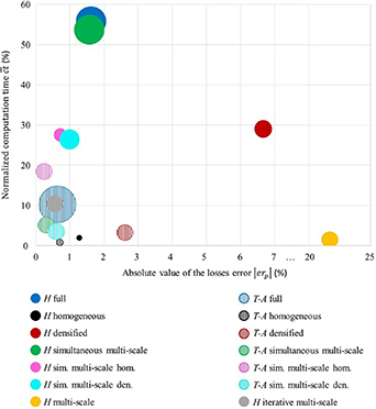
Figure 4. Bubble chart presenting the trade-off between accuracy and computation time. The bubbles closer to the origin are those of the models that better fulfil the compromise between accuracy and computation time. The areas of the bubbles are proportional to the number of DOF. Reproduced from [9]. © IOP Publishing Ltd CC BY 3.0.
Download figure:
Standard image High-resolution imageTable 3. Comparison of different modelling approaches with the H and T-A formulation [9].
| Losses (W m−1) | ct (h) | DOF | |
|---|---|---|---|
| Reference | 127.24 | 31 h 32 min | 563 893 |
| Model | Error (%) |
 (%) (%) | DOF |
| H full | 1.62 | 55.81 | 359 408 |
| H homogenous | 1.28 | 1.94 | 11 838 |
| H densified | 6.67 | 29.03 | 120 424 |
| T-A full | 0.64 | 10.25 | 548 624 |
| T-A homogenous | 0.71 | 0.78 | 20 612 |
| T-A densified | −2.62 | 3.22 | 103 638 |
It was shown that for the T-A formulation (striped bubbles), the homogeneous and the simultaneous multi-scale were within the first square of the grid. It was concluded that these methods have an error of less than 1% and less than 10% of the normalized computation time.
In [11], the implementation of the T-A homogenisation method was achieved for the first time in 3D. The validation of the method was done by experimental analysis of an 86-turn double pancake racetrack coil. For applications such as a racetrack coil where a straight as well as a curved segment of the coil needs to be modelled, 2D simplifications are often not sufficient to accurately simulate the electromagnetic behaviour. The authors concluded that the AC loss of 2D models could show a larger discrepancy if the number of turns was increased. Furthermore, the 3D T-A homogenized model improves in its efficiency as the number of turns increases, compared to other FEM models such as the H formulation. Therefore, this method could be valuable for the numerical analysis of large-scale HTS problems, which cannot be represented accurately in 2D.
In [14], the authors continued their investigation of the homogenisation method in 3D using the T-A formulation. The 3D approach was compared with 2D infinitely long and axial-symmetric models to show the difference in the current distribution as well as the losses. Although a 2D estimation of a racetrack coil is often sufficient, it was shown that there are differences in the penetration of the HTS coil, due to the anisotropy of the critical current. In comparison with the homogenised H formulation the higher penetration in the arc segment of the racetrack coil was validated since the influence of the self-field in this region is higher than in the straight part. The authors had to concede that the H formulation was faster than the T-A formulation, unlike in 2D. Nevertheless, they state that the mode is extremely necessary and will enable the design and optimisation of HTS applications in 3D in the future.
4. Applications
In this section the research conducted using the T-A formulation is reviewed. In power applications, the T-A formulation is of particular interest for the simulation of HTS cables and large-scale magnet applications making use of the advantages from advanced modelling strategies such as the homogenisation method to model large numbers of HTS turns.
4.1. Basic tape and coil modelling
The critical current of superconducting coils was investigated in [15], as this is crucial for the limitation of the performance of the coil. The limiting factors such as temperature, the magnitude and orientation of the magnetic field inside the superconductor were evaluated using H and T-A formulation models. Also, static simulations with the P -model and the modified load-line method were used to estimate the critical current of coils when time approaches infinity. In order to model a superconducting double pancake racetrack coil with more than 200 turns of a 4 mm-wide tape, a 2D infinitely long conductor was considered wherein the circular part was neglected. This was justified by the authors since the critical current of a racetrack coil is determined by the average electric field of the circular and the straight part. When the straight part was longer than the circular part, comparisons of 2D T-A and 3D H formulation models showed a good agreement. Their conclusion listed the T-A formulation as reliable for the estimation of the critical current density, although it overestimated the Jc by 19%. This was assumed to be due to the varying n-values, length uniformity of the critical current and angular dependence, manufacturing process as well as the different cooling efficiency between the short sample, which was used to verify the findings experimentally, and the whole coil.
In [16], the effects of screening current, caused by the penetration of the magnetic field into the HTS tapes was investigated. Two major problems, namely the screening current induced field (SCIF) and the field drift were identified for wound HTS coils. The effects of Jc and the n-value were studied for both problems. Using the T-A formulation and making use of the homogenisation method allowed the authors to run multiple simulations, which would have taken months to simulate with the conventional H formulation. The results showed that a higher Jc causes a higher screening current, while an increase in n-value hinders the relaxation of the screening currents. It was concluded that in reducing both quantities, the two problems were negated, which is contradictory to the use of HTS, since high Jc and high n-values are desired. Other ways of mitigating the SCIF and field drift are the striation of HTS tapes and the current sweep reversal, which are shown to be effective methods. As these methods depend on the coil configuration, they need to be evaluated for each magnet and operating cycle.
The screening current induced strain gradients of a small REBCO pancake coil were investigated experimentally and analytically in [17]. Two coils with a diameter of 150 mm and monofilament and another with 3-striate/4-filament REBCO tapes were tested. A 5 T room temperature magnet was used to excite a strong screening current and further apply a non-uniform Lorentz force to each coil in the experimental setup. The simulations were conducted using the axial-symmetric 2D T-A formulation. At low strain gradients, the experimental results agreed with the numerical solution. The striated multifilament conductor provided a solution to the mitigation of screen current induced strain gradient.
An extension of the T-A formulation model to thick superconductors was proposed in [18], which was used to simulate a racetrack coil with 52 turns. The turns were considered to be either in electrical contact (coupled) or electrically insulated (uncoupled). Three different models, the T-A and H formulation as well as the MEMEP method were used to compare the losses of this stator coil for a superconducting motor. The results showed a good agreement between the methods, only at low currents for the coupled T-A formulation there was a slight discrepancy. This was because in the T-A formulation the coupled tapes are simulated as bulks rather than individual tapes when using the H formulation and MEMEP method. The losses of the coupled case were twice as high compared to the uncoupled case, due to the non-uniform current distribution in the tapes. It was shown that the T-A formulation was advantageous especially for 2D problems that can be approximated as infinitely long or have an axial symmetry.
In [19], the authors implemented the T-A formulation in GetDP. The authors proposed a new derivation of the T-A formulation, wherein global constraints were imposed on the current or the voltage for the individual tapes. It was concluded that the T-A formulation is an efficient formulation to model the electromagnetic behaviour of superconducting tapes.
4.2. Power applications
This section reviews the works implementing different forms of the T-A formulation discussed in section 2 for calculating AC losses in various applications and scenarios.
4.2.1. High current cables.
The T-A formulations have been implemented to compute the AC losses in various types of high current cables which are comprised of HTS tapes.
4.2.1.1. Roebel cables.
In [20], the authors studied the remnant field characteristics of REBCO based 10-strand Roebel cables after removal of the external magnetic field, numerically and experimentally. A 3D FEM model using T-A formulation was built and validated with the measured results mapped out using a Hall probe. They found that the remnant field was dependent on the maximum external magnetic fields and different height with respect to the tape wide surface.
In [13], the authors carried out a performance assessment of T-A formulation against H formulation on AC loss calculation of superconductor, in terms of the number of DOF, computation time and accuracy. A combination of element order for T formulation and A formulation were used, varying from linear to cubic, while first-order curl element and second-order curl elements were considered for H formulation model. Different relative tolerances were investigated as well, such as 3 × 10⁻⁴, 1 × 10⁻⁴ and 1 × 10⁻⁵. Two benchmark models were chosen: a single REBCO straight tape modelled both in 2D and 3D, and a 14-strand Roebel cable modelled in 3D. It was found that in the model of 2D single tape with coarse mesh, the solving time, and the number of DOF were comparable in the T-A and H models set with equivalent element orders. When the mesh was finer, T-A model with linear Lagrange element for T formulation and quadratic element for A formulation was much faster, as compared to H formulation model with curl linear element, although the number of DOF was larger. The 3D T-A model where linear Lagrange element and linear element were set for T and A formulation achieved better accuracy of AC losses. However, it took longer time compared with H formulation model with curl linear element. In the case of the 14-strand Roebel cable, the 3D T-A model with linear Lagrange and quadratic element set for T and A variables was advantageous in terms of time per thousand DOF but required much greater computation memory, as compared to curl linear element H formulation model.
4.2.1.2. CORC® cables.
In [21], the authors studied the influence of harmonic current on transport AC losses of a 10 MW/3 kV 2 kA tri-axial CORC® HTS cable aimed for hybrid-electric aircraft, by means of a 2D model based on T-A formulation. It was observed that under three-phase balanced load and sinusoidal current, the loss in the outer phase could be twice that of the inner phase due to the magnetic field distribution; a small harmonic current (less than 10% of the rated current) could result in a significant increase in AC losses, up to 40%.
Although the 2D model could simulate the electromagnetic behaviour and predict the AC losses of CORC® cable within an acceptable accuracy, the real structure of the CORC® cable was not totally included. Then, a 3D model of the CORC® cable using T-A formulation was proposed and developed to enhance on this.
In [22], to investigate the physical performance of a REBCO based CORC® cable when a hot spot was induced on one tape, the authors developed a 3D multi-physics electro-magnetic-thermal model by coupling four modules, including a T formulation model, an A formulation model, a heat transfer model and an equivalent circuit model. They analysed and discussed the current redistribution among all tapes (figure 5), voltage drop, and temperature variation of the tapes caused by the hot spot, under different amplitude of terminal contact resistance (TCR). It was found that the quench risks of the CORC® cable facing a hot spot could be significantly reduced by minimizing the TCR. With a low TCR, such as Rt < 5 µΩ, the current redistribution mainly depended on the critical current of the tape without a hot spot. With high terminal resistances (Rt > 5 µΩ), the current redistribution mainly depended on the TCR.
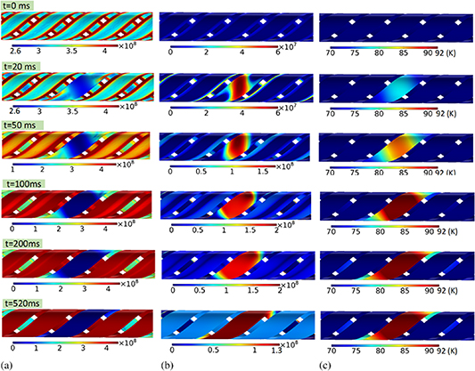
Figure 5. Distribution of the current density in the superconducting layer, metallic layers, and temperature during a hot-spot-induced quench in a CORC® cable. The heat quench was 183 mJ and terminal contact resistance was 100 µΩ. Figure reproduced with permission from [22]. © IOP Publishing Ltd All rights reserved.
Download figure:
Standard image High-resolution imageIn [23], the authors focused on the magnetization loss analysis of CORC® cables by an experimentally validated 3D model using T-A formulation. In particular, the authors studied how the winding direction, multilayer structure and utilization of striation tapes could affect the magnetization loss of CORC® cables. They found that an increase of the number of cable layers could decrease cable losses due to the field shielding effects. For CORC® cables with multiple layers, the magnetization loss was significantly affected by the winding direction and the packing arrangement of air gaps in each layer. In addition, tape striation could remarkably reduce the magnetization loss only when the CORC® cable was exposed to high magnetic fields.
In [10], the authors proposed an accelerated 3D T-A formulation model to study the AC losses of a CORC®-like conductor based on quasi-isotropic conductor. The acceleration of the T-A model was achieved by reducing the solution area employed with T formulation. In other words, the J distributions of some selected superconductors were solved by T formulation and J distributions of other superconductors were approximated by linear interpolation. It was concluded that the pitch length of the CORC®-like cable could significantly affect the current distribution among superconductors and, hence, their AC loss. An optimal pitch length was found with minimized AC losses.
In [24], the quench of a single-layer REBCO-based CORC® cable wound by three tapes with non-uniform terminal contact resistance Rt was investigated. A 3D multi-physics model was built, including three modules coupled with each other, a T-A formulation model, a heat transfer model and an equivalent circuit model. A heat pulse was applied to simulate and initiate a local hotspot on one tape. Current redistribution, voltage, and temperature of each tape during the hotspot induced quench process were reported and compared, when the heat pulse was imposed on the tape with different Rt. It was concluded that for a single-layer CORC® cable with non-uniform terminal contact resistance, when a hotspot was induced on the tape with middle value of Rt, the CORC® cable was most stable due to the highest minimum quench energy.
In [25], the author showed her study on advanced 3D and 2D modelling of HTS CORC® cable with T-A formulation implemented for the electrical propulsion system. The focus of the thesis was to understand how the cable structure affects the electromagnetic and quench behaviour, along with how these effects could be minimized. The author developed and applied T-A formulation to 3D modelling of CORC® cables. T-A formulation demonstrates advantageous in simulating the real structure of CORC® cables to achieve acceptable accuracy by relatively fast speed, as compared to simple 2D model which could not fully represent the complex electromagnetic field coupling due to the real structure, and 3D models using conventional H formulation which could have taken up to months. The 3D model of CORC® cable using T-A formulation allows authors to investigate more critical issues of CORC® cable, including to calculate accurate AC losses, to investigate hot spot-induced quench along the cable, to explore current sharing in different layers of the CORC cable mainly caused by terminal contact resistance, etc.
In [26], the authors studied the CORC® cable loss using a multi-physics electromagnetic-thermal coupled model based on T-A formulation. The model was validated by comparing the transport AC losses of a single tape solely calculated by H formulation, 2D T-A formulation and 3D T-A formulation. The authors proposed an improved 3D T-A model with the functionality of analysing current redistribution between superconducting layer and other metal layers during over current and fault regime, by post-processing the electromotive force E, although the superconductor was regarded as a thin shell in the model.
4.2.1.3. Stacked-tape cables.
In [27], 3D electromagnetic numerical models were built based on T-A formulation, to study the AC loss characterization of CORC® cable, twisted-stacked-tape cable (TSTC), and double coaxial cable, under different transport current and external magnetic field. The effect of pitch length in double coaxial cable inner conducting layer was also discussed. The results showed that AC loss in TSTC cable increased an average of 40% over the other cables, at any transport current, while AC loss in double coaxial cable was 20% lower than that of CORC® cable when exposed to background magnetic field.
In [28], to achieve high current capability of superconductor, the authors proposed a quasi-isotropic straight superconducting strand, and characterized a 35 cm short sample by means of experiment and numerical calculation. The quasi-isotropic strand was comprised of four units, each unit of which was stacked alternatively by 7 copper tapes and 7 HTS tapes with the width of 2 mm. Transport AC losses in the proposed strand were measured under different frequencies ranging from 30 Hz to 200 Hz. Magnetic flux density distribution and AC loss in each HTS tape were also discussed, at peak current of 800 A, 50 Hz. The AC loss results calculated from a 3D T-A model was consistent with the measured ones at frequencies below 75 Hz. At frequencies of 30 Hz, 50 Hz and 75 Hz, the calculated AC loss dependence on normalized current Ipeak/ Ic keeps consistent with the experimental results, but much higher than the Norris strip model, due to two main reasons. One reason is the contribution of eddy current loss in the copper tapes, and the other reason is that each HTS tape in the quasi-isotropic strand is affected by the magnetic fields from other tapes, whereas Norris model assumes a uniform current transporting in self-field. AC losses in the quasi-isotropic stack shows frequency dependency which indicates that the eddy current loss in the copper tapes cannot be neglected.
4.2.1.4. Cables with twisted structures.
In [29], the authors proposed a finite element 2D model of a 5-slots twisted-stacked-tape slotted-core HTS Cable-in-conduit conductor (CICC) using T-A formulation, to investigate the current distribution among tapes in HTS stack(s). The numerical model was validated by the agreement with experimentally measured V–I curves of the CICC. To study the effect of terminal contact resistance Rterm on the current distribution between tapes within stacks, two cases were considered: Rterm was identical for each tape-copper joint, and Rterm showed a statistical distribution, under three experiments: #1 stack of 20 tapes, #2 two adjacent stacks, and #3 a bent stack with bending radius of 0.15 m. It was found that the variation of Rterm could significantly change the initial current distribution within the tapes of stacks. What's more, V–I curves would not change drastically if Rterm was smaller than 500 nΩ. Ic degradation and non-uniform current distribution of the tapes were recorded in the bending stack, which could further lead to thermal instability during operation.
In [30], AC losses in a twisted quasi-isotropic superconducting conductor stacked by HTS tapes and copper tapes alternatively were investigated by 3D simulations based on T-A formulation and experiments. A twisting apparatus was developed to accurately adjust and fix the twist angles of the quasi-isotropic conductor. Critical current and AC loss behaviour under different twist pitch length were measured at 77 K in liquid nitrogen bath. The measured critical current of the twisted conductor tended to degrade with the decrease of pitch length, and a 5% critical current degradation was found when the pitch length was 240 mm. The AC loss of the twisted quasi-isotropic conductor was reduced to 89% and 79% of that in the non-twisted conductor at low frequencies, when the twisted angle was 180° and 300°, due to the uniform current distribution among the HTS tapes.
4.2.2. Fault current limiters.
In [31], the authors focused on the superconducting DC bias coil of saturated iron core superconducting fault current limiter (SIC-SFCL). A multi-objective optimization approach using the Nelder-Mead algorithm for an optimal coil geometry was proposed and presented, with three objective functions: to maximize the critical current density in the HTS tape, minimize the current flowing the DC biased superconducting coil, and minimize the coil price. The SIC-SFCL was simulated by a 2D T-A formulation model in COMSOL, which was validated by measurements of a non-superconducting saturated iron core prototype. The finite element model was coupled with an electrical circuit by electrical lumped parameters, representing the DC bias superconducting coil and AC copper coils. In terms of the coil geometry optimization, the authors showed the normalized critical current density by varying the stack and layers of the biased coil, and the algorithm indicates that fewer layers and more stack number was preferable. The authors also investigated the fault analysis with the optimized biased coil geometry in SIC-SFCL, in the system where steady current was 25 Arms and the peak short circuit current was 1.6 kArms. A-V and T-A formulations were both used and compared to observe the magnetic flux density and normalized current density. It was found that minimal fill factor in the superconducting bias coil was not suitable for minimizing its critical current density.
4.2.3. Electrical machines.
In [32], the authors aimed to establish T-A formulation models to simulate superconducting electrical machines and AC losses in superconducting windings. Firstly, a 2D time dependent model based on T-A formulation was developed to evaluate the AC losses of a specific synchronous motor. The model was further validated by comparing the current density distribution and AC losses with the previously validated results calculated using the minimum electromagnetic entropy production method (MEMEP). The AC losses computed by the two methods had a difference around 5.6%, which indicated a good agreement. After this, the authors added the Jc anisotropy into the model, by incorporating the perpendicular-field-dependent Ic data into the motor model. The AC losses in the stator winding at 65 K and 77 K calculated using the proposed T-A model and MEMEP model showed a difference of 1.5% and 5.6% only, which again proved the accuracy of the proposed model.
In [33], the authors studied the electromagnetic behaviour and AC loss estimation of a 10 MW synchronous generator, in which the rotor was comprised of permanent magnets, and the stator was comprised of superconducting coils, using T-A formulation. To obtain current distribution in stator windings for feeding the T-A formulation model, a resistive model was implemented firstly by connecting a load to the generator; once the induced current distribution was captured, the resistive model was disconnected, and the superconducting model started to compute. Three generator designs (figure 6) were studied and compared: the first one was based on distributed coils wound with 4 mm-wide tape located in the stator with iron teeth; the second design, similar to the first one, had no magnetic teeth but air-gap windings; the third design was similar to the first one, but 2 mm-wide tapes were used instead of 4 mm.
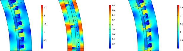
Figure 6. Magnetic flux density norm in tesla for one pole pair of the three generator designs considered in [33], at the beginning of the second cycle of simulation. Figure courtesy of Carlos Vargas-Llanos (Karlsruhe Institute of Technology). See [33] for more details.
Download figure:
Standard image High-resolution imageConclusions were drawn that the slot-less design yielded to uniform current distribution among coils, and thus, losses were dissipated more uniformly. A roughly 44% AC loss reduction was observed in the third design, as compared to the first design. A sensitivity study was also carried out over the frequencies and cryogenic temperatures. A linear increase of losses in kW was observed when the frequency increased at given temperature. Much higher losses were produced in the first and second design when the temperature was above 68 K, whereas the third design showed steady loss performance against temperature variation.
In [34], the authors studied the AC losses in an HTS generator with superconducting coils as rotor, by means of T-A formulation. The model was validated by comparing the results calculated using A-H formulation on the aspects of magnetic flux density distribution of the whole generator and HTS coils area, as well as instantaneous AC loss of the studied field winding. Using the validated model, the effects of the ferromagnetic stator teeth and the shielding layer on AC losses were further investigated, by three cases. Conclusions were drawn that the adoption of ferromagnetic stator teeth could significantly cause sixth-order harmonic magnetic field, hence, increased the AC losses in field winding. Addition of a copper shielding layer at the rotor side could reduce the AC losses in rotor winding in the steady state and also load variation process, but extra attention should be paid on eddy current loss generated in the shielding layer itself.
In [35], the electromagnetic and mechanical properties of a fully superconducting generator were investigated, which was composed of field windings and armature windings made from YBCO superconducting racetrack coils. The moving mesh method was incorporated into the 2D T-A formulation model to simulate the rotating structure of the generator. Virtual tapes were introduced to compute the induced current in armature winding, which was further fed back to the T formulation. The model was validated by comparing the calculated results from H-A model on the aspects of radical gap field, armature current, magnetic flux distribution and total AC losses in the generator windings. In addition, the stress distribution in the rotor half coil was shown and analysed. It was concluded that the AC losses in the armature winding was increased significantly when field currents increased. The body force and stress were concentrated on the boundary of the field winding and armature winding, and the field winding suffered greater stress than the armature winding due to stronger magnetic field.
In [36], the authors studied the electromagnetic and thermal behaviours of a synchronous generator comprised of HTS armature winding by proposing a numerical model which was coupled with three sub-models, including a field model, an equivalent circuit model and a thermal model. AC loss of the armature winding under rated operation was calculated. Transient electromagnetic-thermal behaviour of the HTS coil under a three-phase short circuit fault at the no-load condition was analysed. It was observed that the critical current of each turn of the armature winding was not identical under the fault due to different ambient magnetic field, and this critical current deviation of turns led to different current distribution among layers and various temperature rise. Thermal analysis showed that a thicker copper stabilizer improves the thermal stability of HTS coil upon the fault.
In [5], the authors proposed HTS dynamo as a new benchmark problem for the HTS modelling community, consisting a permanent magnet rotating past a stationary HTS coated conductor wire in an open-circuit configuration. The benchmark was calculated using multiple methods, including H formulation, coupled H-A and T-A formulations, the Minimum Electromagnetic Entropy Production (MEMEP), Integral Equation (IE) and Volume integral equation-based equivalent circuit (VIE). Excellent qualitative and quantitative agreement was observed between all models for the open circuit equivalent instantaneous voltage and the cumulative time-averaged equivalent voltage, together with the current density and electric field distributions within the HTS wire at specific positions during the magnet transit. A critical analysis and comparison with all modelling approaches was presented, regarding key metrics: number of mesh elements in the HTS wire and the entire model, number of degree of freedoms, tolerance settings and the approximate time taken per cycle for each model. The benchmark provided researchers with a suitable framework to validate, compare and optimize their own approaches for simulating the HTS dynamo.
In [37], design, fabrication, and testing of a non-insulation double-pancake racetrack coil for an HTS synchronous motor, which was energized by HTS flux pump, were presented. 2D T-A formulation model was built to simulate the electromagnetic distribution of the double pancake coil. The authors proposed a mechanical way to fix the HTS coil instead of epoxy resin impregnation, due to the concern on different expansion and contraction ratios of HTS tape and epoxy resin that might cause coil damage. Critical current test for the HTS coil was presented at 77 K. A charging test with rotating flux pump was also carried out. The charging test results showed the pump current got saturated once the output DC voltage was consumed by internal resistance.
In [38], a superconducting linear induction pump was analysed, using the T-A formulation to evaluate the AC loss characteristics under self-field and an external alternating magnetic field. The study showed that the AC loss, when a three-phase alternating current was applied, featured a symmetric distribution due to the self-field. The outer coils of the pump generated less AC loss than the ones in the center. When an external alternating magnetic field was applied, the coils at the edges had the highest losses, due to the diamagnetic properties of superconductors.
4.3. High field magnets
Large-scale HTS magnets usually consist of stacked HTS pancake coils. The coils are made of hundreds of turns of HTS tapes, which due to the high aspect ratio of HTS tapes, will result in a large number of elements for the numerical model. Here, the T-A formulation can help to reduce the complexity of the simulation by making use of geometrical simplifications. Applying the thin strip approximation combined with a multi-scale or homogenisation method to simulate a stack of tapes, can significantly reduce the number of elements of the geometry, while keeping the electromagnetic integrity of the HTS coil. It is essential to numerically investigate such large-scale systems before they are built in order to evaluate the performance and potential problems of the magnet.
In his viewpoint, Ainslie [39] identified the screening current-induced magnetic field and its associated stress/strain as one of the major challenges for the design of high-field magnets. This phenomenon was investigated numerically, using the T-A formulation by several researchers.
The influence of shielding/screening current effect in high temperature superconductors was investigated in [40]. The experimental setup consisted of an LTS background magnet providing up to 9 T parallel field and an HTS insert coil. The measured data for the hoop strain of a 10 mm REBCO tape test sample was compared with numerical results using the T-A formulation.
The issue of distorted magnetic fields produced by an induced persistent screening current in the tape under time-varying conditions was studied in [41]. A novel REBCO conductor design, consisting of narrow-stacked (NS) wire, bundling 1 mm wide tapes was used for this study. This design makes use of the fundamental property that a smaller width features a smaller screen-current field (SCF). Using the T-A formulation, this design was analysed numerically and confirmed by experiments. It was demonstrated that the SCF in the NS wire was reduced, and it also met the critical current requirements for applications such as NMR, MRI, and HEP.
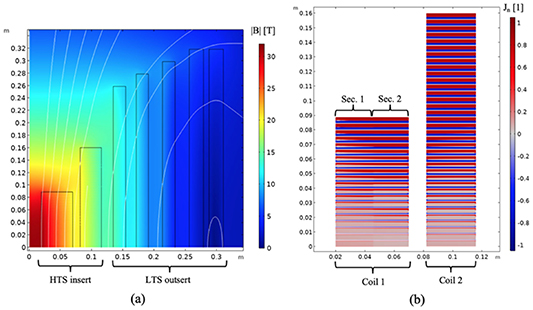
In [42] the screening currents and corresponding hysteresis losses in the 32 T all-superconducting magnet of the National High Magnetic Field Laboratory (NHMFL) were investigated. This magnet was tested in 2017 and consisted of HTS insert and LTS outsert magnets, which produced a total magnetic field of over 30 T. The challenge was to model the 20 000 turns, which was tackled by using the homogeneous T-A formulation (figure 7). A comparison with other numerical models (homogeneous and multi-scale H formulation) showed that it was possible to significantly reduce the computational load of the simulation. Therefore, it was possible to model a full-size HTS insert and include the background field of the LTS outsert magnet. The whole simulation was achieved within hours using a desktop computer.
Figure 7. (a) Magnetic flux density magnitude and (b) normalized current density at 1 h, the first peak of the ramping cycle. The upper pancakes are fully penetrated by screening currents. Figure reproduced with permission from [42]. © 2020, IEEE. Reprinted, with permission, from [42].
Download figure:
Standard image High-resolution image
The T-A formulation was used in [43] for the simulation of 40 REBCO pancakes with 12 000 total turns, which produced a field of 15 T. Due to screen current induced field (SICF), it was shown that the field in the centre of the magnet was reduced significantly. The investigation of the mechanical stability and safety of the high field magnet showed the risk of high residual fields at the top and bottom of the magnet coils. Since the top and bottom coils had a higher radial field than the centre coils, the induced screening currents and magnetization loss were increased. Furthermore, during ramp cycles, the magnetization loss was increased due to the screening currents generated by the superconductor. By using an equivalent turn model with the T-A formulation, the number of turns that needed to be modelled was reduced, while keeping the same electromagnetic performance. This approach was validated by simulations using the H formulation.
In [44] a HTS synchronous driving system for an EDS (electrodynamic suspension) train was studied. The authors computed the propulsion force under different operating conditions analytically and numerically using the T-A formulation for a REBCO magnet. It was shown that due to the high excitation speed of transport current, the critical current of the coil tends to be underestimated.
The T-A formulation was used in [38], to validate the developed self-consistent model, in order to estimate the critical current of a racetrack REBCO magnet. The evaluated relative error between the models was 0.48% for the whole coil and an identical magnetic field distribution.
A persistent-current superconducting magnet system with solid nitrogen cooling for magnetic levitation trains was proposed in [45]. The superconducting magnets need to cover the vibratory motion range when Maglevs are operated at high speeds >600 km h−1. The field was designed to be >0.8 T using no-insulation 2G HTS wires. These wires feature high in-field current, enhanced self-protective stability and volumetric compactness. The T-A formulation was used to model a 300 turn double pancake coil and evaluate its electromagnetic performance and demonstrate a 2G HTS magnet system for maglev applications.
5. Discussion
The
T-A
formulation gained popularity in the last years due to two main factors. First, the
T-A
formulation is a more efficient numerical method than the widely used
H
formulation, due to the simultaneous computation of two state variables and the continuous exchange of the current density
J
and magnetic flux density
B
. The other is the convenient implementation and user friendliness in FEM software like COMSOL, which is mainly used to run simulations for HTS applications. As pointed out by the authors in [9], setting up a model using the
H
formulation, can be quite time consuming since the transport current is imposed via integral constraints, which need to be defined for each tape individually. In comparison, the
T-A
formulation allows imposing the transport current via Dirichlet boundary conditions at the edges of the tape, which makes it very easy to build. In the case of simultaneous multi-scale models, the transport current just needs to be applied to the analysed tapes. Although this does not simplify the model compared to the full
T-A
model, it is easier to implement than the same approach using the
H
formulation. The easiest models to build are the homogeneous models, as the simplification of a stack of tapes into a homogenised bulk reduces the amount of boundary conditions especially for large numbers of tapes. In the
T-A
formulation, the transport current is still imposed via Dirichlet boundary conditions at the edges, but especially for the
H
formulation, the integral constraint only needs to be defined for each bulk segment, rather than each individual tape. Nevertheless, in order to prevent current sharing, air gaps need to be implemented between the bulk segments when using the  formulation, which complicates the geometrical design. Overall, it can be said that the
T-A
formulation is easier to use, especially for researchers who are not experts in the software.
formulation, which complicates the geometrical design. Overall, it can be said that the
T-A
formulation is easier to use, especially for researchers who are not experts in the software.
This was shown for a wide range of different power applications from high power cables, fault current limiter, electrical machines to high field magnets. Especially in large-scale applications, where the number of HTS tapes is large, the T-A formulation has the efficiency to solve these simulations within reasonable time.
Expanding on the conventional T-A formulation for tapes and making use of simplifications such as the multi-scale or the homogenisation method can further improve the computation time. These methods are validated for 2D and 3D using experiments as well as numerical comparison with the H formulation.
There are limitations to the T-A formulation and the use should be evaluated for each problem individually. Practically all T-A modelling strategies are limited to cases where the thin sheet approximation of the superconducting layer is meaningful [9]. This means that although this modelling technique has a great potential to simulate HTS application simply and fast, there are applications where it is still required to use the H formulation, such as wires with different geometries (MgB2).
6. Conclusion
In this paper the modelling of high temperature superconductors using the T-A formulation is reviewed. In recent years this formulation gained popularity due to its simple implementation and efficient computation speed. By adapting the multi-scale and homogenisation method to the T-A formulation, it is now possible to model large-scale applications with large numbers of turns in excess of the capabilities of other formulations, such as the H formulation. This makes the T-A formulation even more promising for future modelling of HTS.
With these improvements, the T-A formulation was used to simulate the superconducting behaviour in a multitude of applications: high field cables such as Roebel cables, CORC® cables, stacked cables and cables with a twisted structure; fault current limiters, electrical machines, and high field magnets. For these applications the evaluation of AC loss as well as screening currents are of particular interest to researchers.
The main implementation of the T-A formulation is done in COMSOL, a multi-physics software where the electromagnetics can be coupled with a thermal model. Another software that is used to study HTS tapes using the T-A formulation is GetDP.
The T-A formulation has shown to be a reliable alternative to the H formulation. It is especially desired for large-scale applications since the computational speed can be increased tremendously.
Here we reviewed the basic concept and implementation of the T-A formulation as well as the investigation and application to real problems. Although the T-A formulation is suitable and efficient for most problems, there are some cases where it is still necessary to use alternative formulations ( H, T -Ω, H-A, A -V, H -ϕ, MEMEP, P-model, etc) and therefore, the choice of the numerical model needs to be done on a case-by-case basis.
Future works will extend the use of the T-A formulation in 3D to geometries that cannot be accurately represented in 2D. This is especially important for twisted cable and coil configurations, where the homogenous T-A formulation will be a useful tool to enable numerical investigations. Furthermore, coupling of the electromagnetic model with other physical models i.e. heat transfer or mechanical models are of interest when investigating HTS applications.
Acknowledgment
This work was supported by the COST Action CA19108 'High-Temperature SuperConductivity for AcceLerating the Energy Transition' (Hi-SCALE).
Data availability statement
All data that support the findings of this study are included within the article (and any supplementary files).