
Abstract
The fast thermal and electromagnetic transients that occur in a superconducting magnet in case of a quench have the potential of generating large mechanical stresses both in the superconducting coils and in the magnet structure. While the investigation of such quench loads should generally be conducted to ensure a safe operation of the system, its importance is greatly enlarged in the case of high-field magnets based on strain sensitive superconductors. For these, a rigorous analysis of the magnet mechanics during a quench becomes critical. The scope of this work is hence to bring, for the first time, a detailed understanding of the three-dimensional mechanical behavior of a Nb3Sn accelerator magnet during a quench discharge. The study relies on the use of finite element models, where various multi-domain simulations are employed together to solve the coupled physics of the problem. Our analysis elaborates on the case study of the new MQXF quadrupole magnet, currently being developed for the high-luminosity upgrade of the LHC. Notably, we could find a very good agreement between the results of the simulation and experimental data from full-scale magnet tests. The validated model confirms the appearance of new peak stresses in the superconducting coils. An increase in the most relevant transverse coil stresses of 20–40 MPa with respect to the values after magnet cool-down has been found for the examined case.
Export citation and abstract BibTeX RIS

Original content from this work may be used under the terms of the Creative Commons Attribution 4.0 license. Any further distribution of this work must maintain attribution to the author(s) and the title of the work, journal citation and DOI.
1. Introduction
The next generation of superconducting accelerator magnets will turn into a reality the ambitious objective of routinely producing magnetic field levels beyond 10 T for the interaction with particle beams [1–4]. This pursuit of higher magnetic performances translates, however, into novel challenges for the magnet design. In particular, the unceasing increase in the conductor current densities, the growing magnet stored energies, and the presence of large electro-magnetic forces have pushed the boundaries of the magnet conception and its quench protection toward new limits.
For the latter case, we refer to a quench as the abnormal termination of the magnet operation that occurs when a part of a superconducting coil transits irredeemably to the resistive state [5–8]. This phenomenon, which leads to the appearance of a growing electrical resistance that propagates within the coil windings, results into the dissipation of the stored magnetic energy and generates a fast transient in the magnet. So-called quench protection systems are normally employed to safely discharge the magnet when a quench is detected, becoming an essential part of the design.
In what regards the search for new magnetic field horizons, a crucial breakthrough for the recent attainment of larger fields in accelerator magnets has been, undoubtedly, the development of high-performance superconductors capable of operating beyond the limits of NbTi technology [9–11]. New high-field magnets are mostly based on Nb3Sn (niobium-tin) conductors, which present superior critical parameters when compared to NbTi. For instance, state-of-the-art Nb3Sn wires enable the transport of current densities in the non-copper area (J) that are above the value of J = 1000 A mm−2 at 16 T and 4.2 K [10]. Such a remarkable performance ultimately paves the way toward the achievement of record fields in compact magnet units.
One of the most relevant particularities of Nb3Sn technology is, on the contrary, the reduced tolerance to mechanical loads and the brittleness of the material. It is today well-known that the superconducting properties of Nb3Sn present a strong dependence in mechanical strain, as proven by a large variety of experiments [12–33]. In practical terms, the conductor performance is prone to experience an undesired reduction, if the loads in the superconducting coils exceed given tolerable values. This decrease in the current transport capability may happen both in a reversible and an irreversible manner [13, 32, 33]. Although in strict terms either of the reductions should be prevented from happening, the permanent decrease is specially dangerous for magnet operation and must be carefully avoided.
As a result of the importance of this aspect, the mechanical design becomes a key factor in the conception of new Nb3Sn magnets. In the present days, a large majority of the proposed designs entail peak stresses in the coils that are in the range of 150–200 MPa during magnet assembly and operation [4, 34]. These stress values approach, and in some cases surpass, the currently understood limits of the conductor (obtained from measurements in cables and single wires [13–17, 32, 33]). There exists, hence, a reduced margin to additional loads that could promptly appear from other sources.
On the other hand, if the magnet mechanics can be seen as an essential topic for new Nb3Sn technology, perhaps the second most important challenge is related to the magnet protection during a quench. The aforementioned large stored energies and current densities push the requirements on the quench protection toward very stringent targets, where large coil temperatures (limited to 350 K in novel designs) and severe thermal gradients can be reached during a quench transient [34, 35].
From the combination of all the features presented in the two last paragraphs, a new fundamental concern arises for niobium-tin magnets: the possible appearance of peak mechanical loads during the quench, which can put in serious risk the integrity of the strain sensitive superconductor first, and of the magnet structure in general. The origins for these new loads are namely: (1) the localized thermal expansion of the warm parts, which generates thermal stresses in the system and (2) the fast electro-magnetic (e.m.) transient, which creates instead an abrupt change in the e.m. forces. By implication, the analysis of the magnet mechanics during a quench becomes necessary.
In order to give a clear support to this statement, let us briefly review the general approach to what concerns the study of quench transients and their protection. Two main characteristics have historically been considered as the core of the quench protection [36]: (a) the control of the temperature increase happening in the superconducting coils, and (b) the management of the electric voltages generated during the discharge. For these, the community has established solid limits that preserve the magnet integrity during a quench. For example, the allowable maximum voltages depend on the insulation system used, but they are consistently set to guarantee the absence of electrical failure within the magnet components. On the other side, the maximum temperature in the coils is defined in order to avoid the damage of the conductor insulation. Additionally, it is also specified based on experimental tests where a decrease of the magnet performance after high temperature events was noticed. The critical value assumed for new Nb3Sn magnets has been previously mentioned to be 350 K [37]. Unfortunately, the same type of limits have never been proposed for the potentially dangerous mechanical loads that may appear during a quench. The necessary link between the most relevant quench physics and the magnet mechanics remains yet to be established.
With the objective of closing this gap, two-dimensional research works have been published in [38–42]. Though, a full understanding of the magnet mechanics during a quench can be only obtained by means of a three-dimensional analysis, as follows straightforwardly from the 3D nature of quench phenomenon. The complexity of this problem was approached in four references of which the authors are aware [43–46], where two different methods aimed at obtaining a first insight into the topic were presented. With our work, we try to finally complete this development and to provide clear answers about the mechanical implications of a quench event.
The scope of this manuscript is thus to present, for the first time, an exhaustive three-dimensional analysis of the mechanical behavior of a Nb3Sn accelerator magnet during a quench. The analysis is performed via finite element modeling (FEM) techniques, whose use in the design of superconducting systems is well-established. On first instance, a 3D numerical model reproducing the quench propagation [47, 48] and the magnet quench discharge has been developed using ANSYS APDL [49]. This model, which is carefully described in [42, 50], has been validated using a large amount of experimental signals recorded during real tests. In a next step, we profit from the output of this computation to transfer the necessary thermal and electro-magnetic loads (with the help of a standard electro-magnetic calculation) to the magnet mechanical model, also built in ANSYS APDL. The link between the simulations enables the study of the magnet quench mechanics based on a quasi-static approximation.
Our analysis in this text will elaborate on the case study of the new MQXF quadrupole magnet built for the high-luminosity upgrade of the LHC (HL-LHC) at CERN [51]. Its large magnetic stored energy and demanding protection, turns the case of MQXF into one of the most interesting among the new Nb3Sn accelerator magnet designs. In addition, the relevance of the study is increased as these magnets will be part of the first Nb3Sn units ever operating in a particle accelerator, proving the readiness of the technology for the development of future magnets. We specifically present the case where so-called quench heaters (QHs) are employed as the main active protection mechanism. These heaters are used to bring rapidly the largest portion of the superconducting coils to the resistive state, provoking a faster current discharge and more a homogeneous quench load.
At last, we try to provide a path towards a first-order estimation of the quench mechanical effects on conductor performance. The analysis of the peak stresses during the quench, predicted by the simulation, is complemented with dedicated experiments on the electro-mechanical limits of the MQXF conductor [33].
2. The MQXF magnet
An important part of the HL-LHC at CERN focuses on the so-called machine triplet regions. There, a combination of quadrupole magnets are placed at either side of the interaction centers to provide the final strong focusing to the beam. The installation of new units for these magnets (also called low-β quadrupoles) is envisaged as a necessary contribution to the increase in luminosity [52].
The new magnets, designed under the name of MQXF [53, 54] and based on Nb3Sn technology, will replace their today's present NbTi counterparts with the objective of producing a gradient of 132.6 T m−1 in a 150 mm single aperture. As a part of the triplet circuit, they will operate at 1.9 K, and will be powered with a nominal current value of 16.47 kA. The most relevant magnet characteristics are summarized in table 1, where Q1–Q3 and Q2 denote the different MQXF versions in terms of magnetic length.
Table 1. MQXF magnet parameters a .
| Parameter | Unit | |
|---|---|---|
| Coil clear aperture diameter | mm | 150 |
| Magnet (LHe vessel) outer diameter | mm | 630 |
| No. turns in layer 1/2 (octant) | 22/28 | |
| Operational temperature Top | K | 1.9 |
| Magnetic length (Q1–Q3)/(Q2) | m | 4.20/7.15 |
| Nominal gradient Gnom | T m−1 | 132.6 |
| Nominal current Inom | kA | 16.47 |
| Nominal conductor peak field Bop | T | 11.4 |
| Inom/Iss at 1.9 K for RRP/PIT (specs.) | % | 77/79 |
| Ultimate gradient Gult | T m−1 | 143.2 |
| Ultimate current Iult | kA | 17.89 |
| Ultimate conductor peak field Bult | T | 12.3 |
| Iult / Iss at 1.9 K for RRP/PIT (specs.) | % | 84/86 |
| Stored energy per unit length at Inom (Q1–Q3, Q2) | MJ m−1 | 1.17 |
| Differential inductance at Inom | mH m−1 | 8.21 |
| Stored energy at Inom (Q1–Q3)/(Q2) | MJ | 4.91/8.37 |
| Fx / Fy (per octant) at Inom | MN m−1 | +2.47/−3.48 |
| Fθ layer1/layer2 (per octant) | MN m−1 |

|
| Fz (whole magnet) at Inom | MN | 1.17 |
a At the time of preparing this manuscript, an update of the operational parameters for the magnet is being performed.
For the first time in an installed accelerator magnet, the baseline strategy for the quench protection relies in the joint use of CLIQ systems [55] and QHs to ensure a safe magnet response during a quench. The heater circuits are integrated in the outer surface of the coils, and cover the two outermost conductor blocks [56]. Regarding the coil design, it accounts for a total of 50 cable turns wound in two continuous layers around a central titanium pole.
To provide the necessary support to the large electromagnetic forces, and to maintain the conductor design position, the coils are assembled inside a shell-based support structure. This force-restraining structure offers as well the capability of applying a certain mechanical preload to the superconducting coils by means of a system of water pressurized bladders and interference keys [57]. In longitudinal direction, the preload is instead provided by a system of tie rods and thick end plates. The magnet cross section is depicted in figure 1, which highlights the position of the mechanical instrumentation systems installed in the magnet (strain gauges (SGs) and optic fibers).
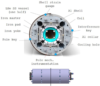
Figure 1. MQXFS magnet cross section and side view. The position of the mechanical instrumentation is indicated by the round markers (in the magnet cross section) and by the vertical line (in the side view).
Download figure:
Standard image High-resolution imageAt the moment of writing this manuscript, the initial R&D phase for the magnet has been almost completed. An extensive campaign for the production of short model magnets (with a magnetic length of 1.2 m and known as MQXFS) has been successfully accomplished, and the test of the full-length magnets has already started. Reports on the measured magnet performances can be found in [58–68].
3. Methodology
The proposed simulation of the MQXF magnet mechanical behavior during a quench is based on a methodology that joins the capabilities of various multi-physics three-dimensional models (see figure 2). The approach relies on the following assumptions:
- (a)The electro-magnetic field problem is decoupled from the rest of the computation [69]. The static magnetic calculation (of standard architecture, not discussed in this manuscript) is used to provide the current-dependent magnetic field and e.m. forces to the other two models.
- (b)A thermal-electric simulation is then used to reproduce the quench onset and the complete magnet discharge. The main objective of this model is to generate the thermal loads and the current profile for the final mechanical simulation.
- (c)The mechanical model reads as a direct input the temperature distribution and the magnet current obtained in (b). The e.m. forces are applied next by using the output of the magnetic code and the quench current. As a result, the analysis of the mechanical behavior through the different steps of the discharge is obtained by means of a quasi-static simulation.
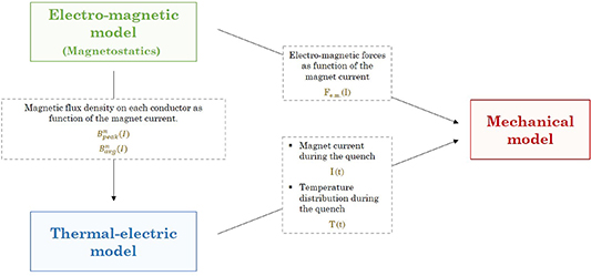
Figure 2. Diagram representing the link between the various models used in our approach. The standard electro-magnetic model will not be discussed in this manuscript.
Download figure:
Standard image High-resolution imageAll models remain fundamentally independent, and the necessary coupling between them is performed by a simple load transfer process between databases. In addition, and although a quench is a fast dynamic transient, the choice for a quasi-static simulation relies on the assumption that inertia and damping effects can be disregarded in the computation.
Our simulation will specifically focus in the case of a quench happening at nominal current, which corresponds to the most relevant scenario for a magnet installed in the machine. With the goal of allowing the model validation with experimental results, we will deal with the available case of a MQXF short model magnet. Finally, and since the protection of the magnet with only QHs corresponds to a conservative scenario (where larger thermal gradients are expected in the coils), we will limit ourselves in next sections to the analysis of this case. Such an exercise is performed in an attempt to prove the presence of enough mechanical margin in the design.
4. Thermal-electric quench simulation
4.1. Model description
In what follows we provide a brief overview on the developed thermal-electric quench model for the self-consistency of this work. An exhaustive description of the model can be found in two earlier manuscripts, which have been published using a graded approach to the problem. In [50], we initially presented the creation of the ANSYS code capable of reproducing the 3D quench propagation in superconducting magnets. In [42], the model capabilities were expanded to introduce the simulation of the complete quench discharge, including the modeling of the most relevant transitory effects [70, 71]. The main characteristics of the computation [72] are:
- The total solution time is divided in small time steps, whose size is adapted depending on the simulation results (adaptive time-stepping).
- The superconducting cable is modeled as a block of homogenized material properties. Direct coupled-field elements are used for the mesh, where the temperature and voltage degrees-of-freedom are evaluated at each time step. Structural parts are instead meshed with pure thermal elements.
- A solving algorithm compares at each time step the current density of all active conductor elements with their corresponding critical value. If the critical value is exceeded, the superconducting element is switched from its superconducting state to resistive.
- The most relevant dynamic effects for a QH protected magnet are included as a power input, i.e. inter-filament coupling losses [42, 71].
- When applicable, the material properties are updated as function of the magnetic field and temperature. The assumptions in the assignment of material properties are explained in [50]. The main sources for the properties are [73–77].
- Adiabatic boundary conditions are assumed in the external surfaces of the models. The heat transfer to the Helium bath is neglected and no magnet re-cooling is considered. For resin-impregnated coil windings, this assumption has been proven accurate for the first seconds of the quench discharge. In figure 3, we compare the average coil temperature inferred from real magnet tests with a simple analytical adiabatic estimate [35]. The good agreement confirms that, for impregnated systems, the stored energy released during a quench protected with only QH is absorbed by the coil enthalpy in a closely adiabatic process.
- To improve the computational times, the magnet discharge is simulated in a thin 3D slab corresponding to a portion of the magnet straight section. Following a multi-stage approach, the detailed three-dimensional temperature distribution in the superconducting coil is then calculated in a separate computation where only the coil is modeled (for this case, the current as a function of time is used as an input and it is obtained from the magnet slab model).
- Full geometry models and their symmetric reduced versions are available. In the case of the MQXF magnet, the quadrupole symmetry allows to perform the simulation of certain cases in just one-octant.
- The QH protection system is carefully reproduced in the thin 3D slab model. The heating stations are meshed and powered using the relevant circuit parameters. This level of detail is avoided in the full coil geometry. In that case, the effect of the magnet protection is accounted by imposing the transition to resistive state of the turns, respecting the delays obtained from the slab model.
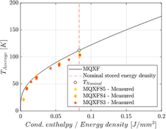
Figure 3. Average coil temperature as function of the magnet stored energy density or conductor enthalpy. The solid line corresponds to the analytical adiabatic estimate and the markers show the experimental extracted values from quenches protected with only QH. The good agreement between both confirms that the released stored energy is, in practical terms, completely absorbed by the coil enthalpy.
Download figure:
Standard image High-resolution image4.2. Model validation
The thermal-electric model has been validated using a large amount of experimental data from the tests of short MQXF model magnets. Figure 4 compares the model predictions, in red, with the magnet current signals obtained from controlled quench discharges. These discharges were provoked by the manual triggering of the QH protection system. The numerical integration of the curves, which receives the name of quench integral when it is performed for the square of the current [78], confirms that the model is capable of reproducing the measured results with a precision of 8%. On the other hand, figure 5 tackles the case of specific tests on the QHs performance. The quench delays are defined as the time required to quench the first cable turn below the heaters, and constitute a measurement of the protection effectiveness. Since the various short model magnets account for slightly different conductor properties that fluctuate around the reference project values, the results are compared with a simulation performed using the nominal conductor. The simulation predicts the delays within a discrepancy of 1 ms at operational current (high-field QH), and confirms that the code is able to reproduce the relevant thermal physics in the magnet.
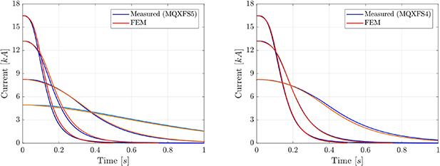
Figure 4. Comparison of the model predictions with experimental signals for different controlled quench discharges in two MQXFS magnets. The left plot shows the case of MQXFS5 (with four tests performed at 16, 13, 8 and 5 kA), while the right plot shows the one of MQXFS4 (with three tests performed at 16, 13 and 8 kA). The blue color is used to indicate the measurements, the red curves show the corresponding simulation results.
Download figure:
Standard image High-resolution image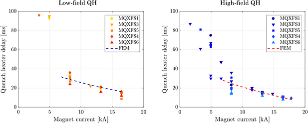
Figure 5. Delays to quench measured from the moment the heaters are powered. Markers show the experimental results, and the dashed lines depict the values obtained from the simulation. The results are grouped according to the QHs position: the left plot corresponds to tests performed in the low-field block, the right to the high-field one.
Download figure:
Standard image High-resolution image4.3. Reference nominal quench results
The results from the simulation of the reference nominal current quench are shown in figure 6. We will extensively deal with the quench mechanics for this case in the next section of the manuscript. The quench location has been voluntarily assigned to the peak field conductor in the center of the magnet (to get the largest maximum temperature), and a total time of 15 ms was assumed for the detection and validation of the quench. The reference MQXF conductor specifications were considered.
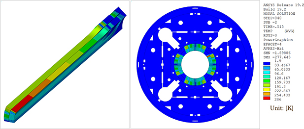
Figure 6. Temperature results from the simulation of a reference quench happening at nominal current. The left plot shows the symmetric 3D coil geometry, where the insulation and the winding pole are hidden for visualization purposes. The right plot shows the same simulation performed using the 3D thin slab.
Download figure:
Standard image High-resolution imageThe contour plots present the temperature distribution at the end of the discharge using the thin 3D slab model (right) and the 3D coil model (left). The latter considers just one half of the quenching coil, where adiabatic boundary conditions are assumed for the symmetry planes. Such a modeling strategy reduces the computational costs at the expense of neglecting the heat propagation to the other half of the coil and to the neighboring components. Given the fact that a standard quench is not a symmetric event, the mentioned simplification needs to be carefully considered. The validity of this approach (for the study of the magnet mechanics during a quench) will be explained in section 5. Note, nevertheless, that as mentioned in the previous section of this manuscript, the magnet discharge is always computed in the thin slab model of the full magnet. The 3D coil geometry just provides the three-dimensional temperature distribution including the effects of the longitudinal quench propagation.
Interestingly, the slab computation shows a 6 K larger temperature for the hot-spot conductor. This is attributed to the presence of longitudinal heat propagation in the 3D coil, which is neglected in the thin simplification. The magnet is practically discharged after 515 ms, showing a final maximum temperature of around 286 K. The average temperature of the system is as well the largest at this point. Regarding the absolute peak value attained during the quench, it is close to 300 K and happens before the completion of the energy dump (the posterior decrease to 286 K is caused by the heat conduction within the coil volume). It is convenient also to highlight that due to the fast nature of the transient and due to the coil insulation, the structure remains ultimately cold through the discharge (see figure 6 (right)). By implication, the assumption of an adiabatic coil is, as already described, a fair strategy for small time intervals and allows to disregard the structure in the 3D simulation.
5. 3D mechanical quench simulation
5.1. Model description
Both two-dimensional and three-dimensional mechanical models were developed for MQXF well before this work (see figure 7), and extensively validated during the test campaign of short model magnets [79–88]. Structural elements are used to mesh the different magnet components, where the geometry of the conductor blocks (composed of many cable turns) is simplified as a homogenized solid volume. Isotropic material properties as function of the temperature are assumed for the different constituents, including for the coils [89] (see table 2). In general, frictional contact elements (µ = 0.2) are set in the interfaces between the different magnet parts, with the exception of the coil components. These are assumed to remain bonded due to their impregnated state.

Figure 7. 2D and 3D MQXF mechanical octant models. The dashed lines show the symmetry boundary conditions, while the colors denote the different materials. A full 2D model has been used to verify the impact of the symmetric approximation.
Download figure:
Standard image High-resolution imageTable 2. Coil block mechanical properties.
| Unit | ||
|---|---|---|
| Material Model | Linear Isotropic | |
| Young's Modulus | GPa | 20 |
| Poisson's ratio | 0.3 | |
| Thermal Strain (293–1.9 K) | 3.9 × 10⁻³ |
Like the previous models, the mechanical simulations profit from symmetry boundary conditions to reduce the computational costs. It is however well-known that most of the quench scenarios in a real magnet are clearly non-symmetric, and there exists usually a hot-spot where the quench starts. We could verify, using the 2D full magnet model, that the general mechanical analysis of all cases as symmetric leads to a small overestimation of the coil peak stresses during a quench (in the order of 6% for a quench at nominal current). Thus, proving that the fastest and simplest simulation lays in the conservative side. This result can be explained by the fact that for the octant case, the hot-spot results to be symmetrically expanded in the magnet and creates a larger mechanical load in all coils. In other words, instead of the case of a single coil initially quenching at a given position, the symmetric simulation reproduces the case of the four coils quenching at equivalent positions (in both halves). The global temperature, and therefore the thermal expansion of the coil-pack, results to be larger and generates larger stresses in the system. We will limit ourselves to the study of such conservative symmetric cases.
5.2. Model validation
The good agreement obtained for the quench discharges in terms of simulated and measured current does not necessarily imply that the predicted coil temperature is correct. If this is not the case, the outcome of the mechanical simulation may not provide reliable information on the quench mechanics. To prove the correctness of our results, we have carried out a detailed campaign for the model validation. The study profits from the installed mechanical instrumentation and concentrates in the analysis of controlled quench discharges (those shown in figure 4 (left)).
5.2.1. Experimental mechanical readings during a quench.
It has been already introduced in section 2 that two different types of strain sensors were used along the tests of short model magnets: resistive SGs and fiber optic sensors based on fiber bragg grating. The positions where the systems are installed correspond to the coil winding poles, the outer shell and the longitudinal tie rods (see figure 1). The measurements rely on active compensation schemes, which seek to remove from the strain readings the apparent effects derived from the magnet operation at cryogenic temperature, and from the presence of high magnetic fields (the last, just applicable for the electrical SGs) [90–93]. When compensated, the main objective of the mechanical instrumentation is to study the magnet response during the assembly and powering phases. Nonetheless, if well-synchronized signals at high acquisition rates are available (we have found consistent results in the range of 100 Hz–2 kHz), the analysis of the magnet mechanical behavior can be also expanded to quench events.
In this latter case, it is essential to consider that the outcome from the measurements will be accurate just up to the first instants after the discharge. The main reason behind it is that for fast quench transients, the thermal gradients remain concentrated inside the coils for a small initial time frame. The structural parts and the compensation system remain, meanwhile, almost at a constant temperature (proven by the thermal model and the signals from the active gauges and compensators). In this regime, there is no imbalance between the main sensor and the compensator, and the readings are meaningful. For larger time scales, the magnet enters into a slow transitory phase of re-cooling where the compensation strategy may result in false strain readings. The data used in our analysis is highlighted in green in figure 8. Note that electro-magnetic transients (including induced currents in the SG electrical grid) cannot be discarded, but they may only affect the SG results.

Figure 8. Azimuthal and longitudinal winding pole stress for a training quench in MQXF. The solid blue line depicts the SG readings, and the dashed red line the corresponding FBG response. The 'quench delta' is highlighted by the black arrow.
Download figure:
Standard image High-resolution imageFigures 8 and 9 show the example of the experimental azimuthal and longitudinal stress seen in the MQXF winding pole (one coil) during a training quench. The values have been derived from the strain measurements assuming a bi-axial stress state and, for a better reading, the time has been set to zero at the moment the quench protection is triggered (t = 0 s). The agreement between both systems, whose readings are found to remain within a difference of ±3 MPa for  s, provides a strong confidence in the results. It should be emphasized that the principles of strain measurements by electrical gauges and optic fibers are completely different, and each of the system is affected in a different way from the relevant quench physics. In fact, and unlike the optic fibers, the SGs show an unexplained response during the neglected re-cooling phase that is under investigation.

Figure 9. Detailed zoom (from figure 8) for the azimuthal and longitudinal winding pole stress during the fast quench discharge.
Download figure:
Standard image High-resolution imageRegardless of the system used, we introduce the concept of the 'Quench delta' as the stress difference between the beginning of the magnet powering and the end of the quench discharge (depicted by the black arrow in figure 8). This delta can be understood as the additional stress that arises from the quench thermal gradients and the fast e.m. transient. Thereby, it can be used as a parameter to characterize the magnet mechanical response during a quench event. Figure 10 shows the correlation between the quench delta values obtained with electrical SGs and optic fibers, for quenches where both instruments were installed together. The plot, which shows a slope of 0.991 for the linear fit and a consistent range of 3 MPa, clearly supports the fact that the delta is a true physical effect and not an artifact of the systems.
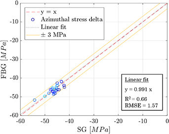
Figure 10. Comparison between the quench delta values measured by SGs and optic fibers for several quenches. The fit information is shown in the right box, where RMSE stands for 'Root Mean Square Error'.
Download figure:
Standard image High-resolution image5.2.2. Comparison with modeling results.
The measurement of the azimuthal and longitudinal strain in the winding pole constitutes the closest place to the conductor, where mechanical strain can be practically measured. Finite element simulations confirm that during the assembly and powering steps, the stress in the winding pole is representative of that of the pole turn cable. Due to the proximity to the thermal gradients generated during a quench, these measurements offer a great possibility to validate the model.
We therefore center our attention on the values obtained for the quench delta in azimuthal pole stress (where the largest load is observed). Figure 11 shows the corresponding results from different MQXFS controlled discharges (measured in one magnet) and their 2D & 3D simulations. Two different modeling strategies are included:
- (a)In the first, displayed with empty markers, the connection between the coil and the pole is modeled as glued (or bonded). This is an usual assumption due to the presence of coil impregnation.
- (b)The second, instead, is represented with full markers and assumes that the coil is allowed to separate from the pole (sliding restricted). This option has been checked, since a detailed look into the pole stress readings seems to indicate that in reality the conductor may experience a de-bonding process due to the large electro-magnetic forces [85].
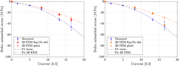
Figure 11. Comparison between experimental and simulated values for the quench delta in azimuthal pole stress. In the left plot the results from the two-dimensional simulation are shown. The right plot depicts instead the case of the three-dimensional model. For the experimental values, the range between the four coils is indicated. Dashed lines represent the quadratic fit of the data.
Download figure:
Standard image High-resolution imageInterestingly, a larger quench delta can be perceived for the second model, as soon as the current level is enough to cause the separation from the pole (seen in the plots at 16.47 kA, where the two simulations diverge). The effect is stronger in the 3D model, which predicts a larger separation than the 2D. The better agreement with the test results, henceforth suggests that the de-bonding mechanism is present in the real magnet. A fact that is consistent with the experimental evidences cited in (b). Nevertheless, the measured delta hints that the de-bonding may happen following a more gradual mechanism. The tests do not experience a sudden change at nominal current as the model suggest (see figure 11 (right), the case where separation is allowed suddenly deviates from the glued one at 16.47 kA). In view of the complexity in accurately simulating this very specific process, we will from now on exclusively focus on the results of the standard glued model and we leave the case where separation is allowed to future studies.
For the bonded case, the simulation yields a very similar result both in 2D and 3D (left and right plots of figure 11). Still, a certain discrepancy is found between the computation and the experimental results. The larger difference is found at nominal current. The glued simulation predicts a delta of 30 MPa, whereas the measured value in the four coils ranges from 36 to 51 MPa. The impact of the coil material properties [72], and the variability in coil geometry [87, 88] are likely to cause part of the difference.
Despite the deviation, the model reproduces correctly the observed magnet mechanical response. The simulation and the experiments show a quadratic dependence of the quench delta with the magnet current. This finding points out that the additional azimuthal stress seen in the winding pole is ultimately driven by the stored energy level. The highest the average coil temperature becomes, the larger quench delta is obtained due to the coil thermal expansion.
To conclude the validation, we consider the analysis not only of the azimuthal pole stress but of all signals available. In figures 12–15, the test results for the discharge at 16.47 kA are compared with their corresponding simulated response. The current profile for this specific quench is presented in figure 12, while the rest of the plots show the stress variation from the moment the current is injected for the winding pole, shell and tie rods. Magenta markers are used to highlight the beginning of the ramp, the red color is used for the point at which nominal current is reached and the black marker depicts the end of the quench discharge. The measurements and the simulation show a small impact in the shell and rods stresses during the quench. The majority of the quench load is, as expected, seen by the superconducting coils. A detailed description of each particular case is found in the caption of the figures.
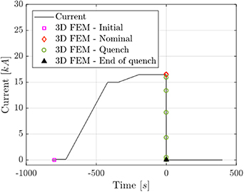
Figure 12. Measured and simulated magnet current. Magenta color is used to highlight the initial condition, the red color indicates the value at nominal current and black shows the end of the quench discharge.
Download figure:
Standard image High-resolution image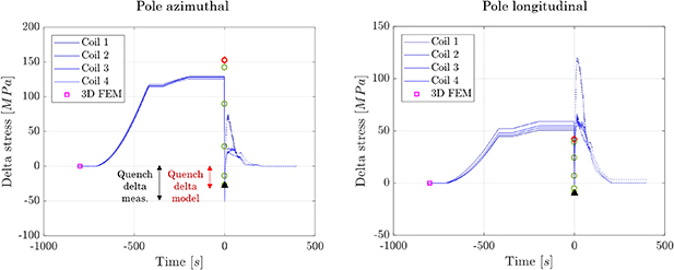
Figure 13. Delta in pole azimuthal and long. Stress for the controlled quench discharge at nominal current. Blue lines show the experimental results for the four coils, while the markers depict the results from the simulation. The color code is consistent with figure 12. Arrows show the FEM and measured delta.
Download figure:
Standard image High-resolution image
Figure 14. Delta in the shell azimuthal and long. stress for the same case presented in previous figure. In azimuthal direction, the model overestimates the delta due to powering. However it still predicts a very small stress increase during the first ms after the quench (first green marker above the red one), in line with the experimental evidences. On the contrary, the posterior decrease is not observed in the test results.
Download figure:
Standard image High-resolution image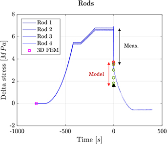
Figure 15. Delta in longitudinal stress measured at the tie rods. Although the model predicts a lower stress variation due to powering, the delta during a quench keeps the consistency with the measurements (arrows). A small adjustment in the friction coefficients can be used to improve the agreement.
Download figure:
Standard image High-resolution image6. Coil peak stresses during the MQXF reference quench
In last section, we have profited from the available mechanical instrumentation to successfully validate our methodology. All the signals analyzed were obtained from the different magnet structural components where the sensors were installed. However, no information on the mechanical behavior of the superconducting coils has been yet revealed.
The 3D bonded model is used here to study the detailed response of the superconducting coil blocks during our reference quench case (explained in section 4.3). This analysis provides the most relevant information for magnet designers. We will focus on the resulting stress state at the end of the quench discharge (t = 515 ms), which corresponds to the instant just before the re-cooling process starts. At that time step, all the stored energy has been released by Joule effect within the coils and the largest stresses have been found. To accurately reproduce the full process, the 3D simulation follows in sequential order all the stages of magnet assembly, cool-down, powering and quench discharge. In addition, and since the magnet preload level has a direct impact in the mechanical behavior, the baseline MQXF target has been considered. It is defined by a measurable azimuthal stress in the coil winding poles of 110 MPa at cryogenic temperature. In longitudinal direction, it is established by the axial pre-tension of the tie rods with a force that corresponds to 100% of the expected e.m. load [84].
6.1. 3D coil stress state
The highest stress values during the magnet assembly and operation phases are identified, for the MQXF coils, in azimuthal direction ( ). Hence, the analysis of the quench loads in this direction becomes of special interest. Figure 16 shows the azimuthal stress distribution in the superconducting coil blocks at cryogenic temperature (left) and after the quench (right). The contour plots show a clear increase that becomes maximum in the position where the hot-spot temperature is located,
  MPa. The effect is more visible when reviewing the results from the subtraction of the cool-down stresses to the quench case (figure 17). For the conductor block in contact with the pole, the increase in stress is in the order of 20–40 MPa.
Figure 16. Coil azimuthal stress distribution after magnet cool-down (left) and at the end of the quench discharge for the reference event at nominal current (right). The effect of longitudinal quench propagation is clearly visible in the plot. The location of the peak stress corresponds to the position where the temperature is higher.
Download figure:
Standard image High-resolution image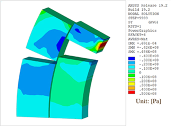
Figure 17. Azimuthal stress difference between the quench case and the cool-down values in the hot-spot region.
Download figure:
Standard image High-resolution imageThe peak Von-Mises equivalent stress predicted by the model is instead very similar for the magnet cool-down and quench steps (σeqv = 140 MPa), and it is located in the coil ends. The effect of the quench loads in σeqv is visible in the hot-spot region where a maximum increase (Δσeqv ) of 27 MPa is found in the block corner.
The radial stress distribution is represented in figure 18. A compressive stress of about 60 MPa is uniformly distributed in the coil outer layer due to the thermal expansion at the end of the discharge. The peak value, 75 MPa, is found close to the position where the hot-spot is located. Similarly to the case of  , the stress delta due to quench is noticeable; Δσr
for the outer coil surface is in the order 15–50 MPa, while for the hot-spot location is of about 70 MPa. In both cases, the high values are motivated by the low stress levels after cool-down.
, the stress delta due to quench is noticeable; Δσr
for the outer coil surface is in the order 15–50 MPa, while for the hot-spot location is of about 70 MPa. In both cases, the high values are motivated by the low stress levels after cool-down.
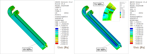
Figure 18. Coil radial stress after magnet cool-down (left) and at the end of the quench (right). The frontal view highlights the peak value, found close to the hot-spot location.
Download figure:
Standard image High-resolution imageWith special emphasis in the coil ends, the last part of the analysis deals with the study of longitudinal stresses. Figure 19 shows the different distributions observed for both simulation steps. A compressive stress increase (Δσz ) as large as 100 MPa is predicted by the model in specific points of the hot-spot region. It is nevertheless important to mention, first, that the stress at cryogenic temperature is again very low there. And second, that the isotropic coil properties assumed in the computation are likely to cause a certain error in the longitudinal results. The authors are aware of different works where the anisotropic behavior of the coil material properties has been presented [89, 94, 95]. This point will be further addressed in next studies. The peak longitudinal stress after the quench is located in the coil ends, and equals 129 MPa.
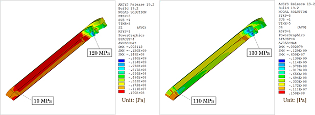
Figure 19. Coil longitudinal stress after magnet cool-down (left) and after the quench (right).
Download figure:
Standard image High-resolution image6.2. Stress gradients
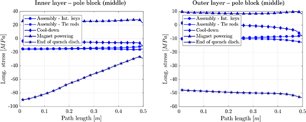
It is interesting to take a look at the stress variation along a certain path, to get an insight into the stress gradients generated during a quench. The case of the coil straight section, where the temperature variation is larger, is particularly revealing here. Figure 20 shows the azimuthal stress along the longitudinal axis of the magnet, for the inner and outer layer conductor blocks in contact with the pole (middle point of the block). The simulation of the magnet assembly and powering steps are added for comparison. Furthermore, the corresponding 2D computation of the same quench is included by means of a red star marker. There exists a 30 MPa gradual increase in azimuthal stress, which follows the quench propagation and coil temperature in the inner layer. Still in this layer, far away from the hot-spot, the values become very similar to the cool-down phase (figure 20 (left)). For the outer coil blocks, where the QHs are placed and the temperature is more homogeneous (no hot-spot), the thermal expansion of the coil rather results in a constant increase of about 20 MPa when compared to the previous steps (figure 20 (right)).
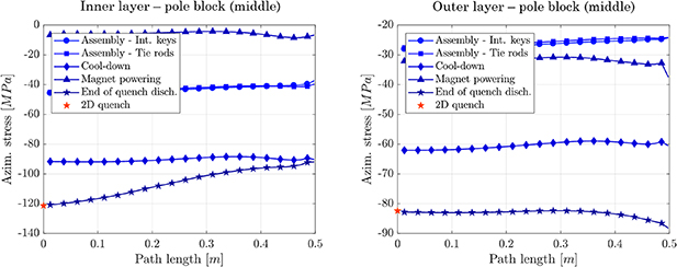
Figure 20. Modeled azimuthal stress along two different paths defined through the straight section. They are located in the middle of the inner and outer layer conductor blocks in contact with the pole. The red marker adds the result from the 2D simulation.
Download figure:
Standard image High-resolution imageAt last, figure 21 shows the same type of analysis for the longitudinal stress. Despite the fact that the peak value is lower, the model unveils the largest gradient in longitudinal direction. Closely following the temperature distribution (figure 21 (left)), a stress variation of 60 MPa is shown by the model. Such a behavior can be explained in a similar way to the azimuthal case. The coil experiences a relevant compression due to its high thermal expansion and due to the presence of the support structure, which remains cold at the end of the fast discharge.
Figure 21. Results for the longitudinal stress along the paths presented in figure 20. The quench creates the highest stress gradient in this direction. The largest delta with respect to the cool-down is identified in the magnet center (90 MPa), and differs slightly from the value reported in the text (100 MPa) due to the path position.
Download figure:
Standard image High-resolution image
6.3. Discussion
In view of the importance of maintaining the stress levels in Nb3Sn coils below safe values, we have centered our study in the coil state at the end of the quench. Although not shown, the magnet structural components have been found to remain within their corresponding stress limits.
Under the modeling assumptions, the 3D mechanical simulation confirms that new peak stresses appear in the superconducting coils during a quench. These stresses are the result of the coil thermal expansion and the change in electro-magnetic forces. Since the coil insulation and the extremely fast nature of the transient prevents the heat to diffuse into the magnet structure in the course of the first instants, the latter remains fundamentally cold. In these circumstances, the maximum coil stresses are obtained at the end of the discharge, when the global coil temperature is the highest and the electro-magnetic forces are almost zero. The same behavior was observed in the reviewed experimental measurements.
In such regime, the quench loads act as a new contribution that adds to the magnet initial condition at cryogenic temperature. For the investigated case at nominal current, the most relevant increase (reaching the largest coil stresses) happens in azimuthal direction and sums the contribution of 20–40 MPa at the hot-spot location (16%–20% of the magnet preload at cold). These results have a profound impact in what regards the correct performance of MQXF magnets. We have succinctly mentioned in section 2 that the applied magnet preload defines the initial coil stress before operation. This in turn implies that if a large preload is chosen, the peak during a quench may approach dangerous limits. For instance, if the target is set to 140 MPa in the pole azimuthal stress at cryogenic temperature, the peak in the coil ( ) at the end of the quench becomes 170 MPa. Special care needs to be taken if an iteration on the magnet preload is performed.
It is also worth to highlight the different time scales for the various phenomena involved. On the one hand, the duration of the multi-physics quench discharge corresponds to approximately 500 ms for an event at nominal operation. During this fast transient, the magnet current decreases, the temperature in the system is increased and, simultaneously, the coil stress state suffers a substantial modification. On the other hand, once the magnet energy has been completely discharged, the posterior re-cooling phase is a much slower process that happens over several minutes.
To conclude, a first-order analysis on whether a given quench stress value can lead to the degradation of the conductor performance can be obtained by comparing the model predictions with the corresponding stress limits of the superconductor. To do so, one needs to carefully test the conductor performance in conditions that are representative to those in a magnet. Taking into account that the highest stresses happen in the direction perpendicular to the conductor's broad face, the most relevant experiments corresponds to so-called transverse tests. In these, an impregnated superconducting wire or cable is subjected to the action of transverse compressive forces. We have carried out, in parallel to the simulation, an extensive campaign for the electro-mechanical characterization of the MQXF superconducting wire [33]. The results from the wire measurements are consistent with the absence of degradation seen during the test of short model magnets and with our obtained simulation results. A deeper look into the effect of the quench loads in conductor performance can be obtained by expanding the analysis using, for example, the proposal published in [96].
7. Conclusions
This manuscript presented the development of a methodology aimed at studying the three-dimensional mechanical behavior of a superconducting magnet during a quench. The analysis becomes necessary for the next generation of accelerator magnets based on Nb3Sn, in order to guarantee the correct performance of the system and the absence of conductor degradation. As a proof-of-principle, we specifically tackled the case of the new HL-LHC MQXF quadupole magnet protected with QHs. The outcome of the work can be condensed into four main results:
- (a)The simulation confirms that new peak stresses can appear in the superconducting coils of a magnet during a quench. Under the modeling assumptions and for the studied case, they are the result of the coil thermal expansion inside the magnet structure (which remains fundamentally cold) and the fast transient in electro-magnetic forces.
- (b)The largest peak stresses are found at the end of the quench discharge, when the magnet stored energy has been completely released. There exists a correlation between the 3D coil stress and the temperature distribution resulting from the quench propagation.
- (c)All the different models employed in our methodology could be successfully validated. The good agreement found with experimental data provides the necessary confidence in the simulation.
- (d)For a quench happening in the MQXF magnet center (at nominal current and with a 15 ms propagation time), an increase in azimuthal stress of 20–40 MPa in the hot-spot area is predicted by the model. Following the quench propagation, the largest stress gradient in axial direction is however seen for longitudinal stresses. A gradual variation of the order of 60 MPa is identified for the inner layer conductor pole block.
Data availability statement
The data that support the findings of this study are available upon reasonable request from the authors.