

Abstract
This paper presents experimental results on a quench of an intra-layer no-insulation (LNI) (RE: rare earth)Ba2Cu3O7−δ (REBCO) coil in a 31.4 T central magnetic field and simulated results on the quench. We have been designing a persistent-mode 1.3 GHz (30.5 T) nuclear magnetic resonance (NMR) magnet with a layer-wound REBCO inner coil. Protection of the REBCO coil from quench is a significant issue and the coil employs the LNI method to obtain self-protecting characteristics. We conducted high-field generation and quench experiments on an LNI-REBCO coil connected to an insulated Bi2Sr2Ca2Cu3Ox (Bi-2223) coil under a background magnetic field of 17.2 T as a model of the 1.3 GHz NMR magnet. The coils successfully generated a central magnetic field of 31.4 T. Although the LNI-REBCO coil quenched at 31.4 T, this quench did not cause any degradation to the coil. A numerical simulation showed the current distribution during the quench was non-uniform and changed rapidly over time due to current bypassing through copper sheets between layers, resulting in faster quench propagation than in an insulated REBCO coil. During the quench propagation, the peak temperature (Tpeak) and the peak hoop stress BzJR (σθ,peak) were calculated to be 330 K and 718 MPa, respectively. These are below critical values that cause degradation. The simulation also showed that the high electrical contact resistivity (ρct) of 10 000 µΩ cm2, between REBCO conductors and copper sheets in the LNI-REBCO coil winding, played an important role in protection. When ρct was as low as 70 µΩ cm2, the quench propagation became too fast and large additional currents were induced, resulting in an extremely high σθ,peak of 1398 MPa, while the Tpeak was as low as 75 K. In short, the high ρct in the present coil caused a high Tpeak, but succeeded in suppressing σθ,peak and protecting the coil from the quench.
Export citation and abstract BibTeX RIS

Original content from this work may be used under the terms of the Creative Commons Attribution 4.0 license. Any further distribution of this work must maintain attribution to the author(s) and the title of the work, journal citation and DOI.
1. Introduction
Development of high-field magnets using high-temperature superconductor (HTS) tapes has been an active field of research for some time [1–13]. Such magnets generally employ the pancake-winding method [14] since thin tape conductors are suitable for winding as pancake-stacked solenoid coils. However, considering the persistent-mode operation required for nuclear magnetic resonance (NMR) magnets and MRI magnets, layer-winding [14] is preferable because longer HTS tapes have a smaller number of superconducting joints and those joints can be installed over the coil where external fields are low. We have been developing a persistent-mode 1.3 GHz (30.5 T) NMR magnet with a layer-wound (RE: rare earth)Ba2Cu3O7−δ (REBCO) HTS inner coil [1]. One of the important technical issues of such a high-field REBCO coil operated at a high current density is protection from burnout due to quench (or thermal runaway). To protect a layer-wound REBCO coil from quench, in previous work we proposed a novel winding method called 'intra-layer no-insulation (LNI)' [15] based on the no-insulation (NI) technique [16–18].
The LNI method resolved the extremely long charging delay of a simple NI layer-wound coil [19, 20]. The LNI method uses pairs of an insulator sheet and a copper sheet as inter-layer materials in an NI layer-wound coil, as shown in figure 1. This winding structure produces a NI state inside each layer, providing a self-protecting behaviour from quench, and electrical separation between layers, resulting in a quite short charging delay.
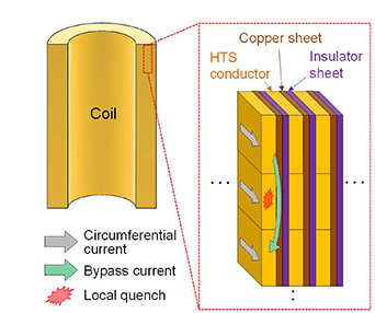
Figure 1. Schematic view of an intra-layer no-insulation (LNI) coil.
Download figure:
Standard image High-resolution imageIn a previous paper, we demonstrated that an eight-layer LNI-REBCO coil was self-protected from quench at a high conductor current density of >700 A mm−2 in a self-field. However, the self-protection behaviour of an LNI-REBCO coil having many layers in a high magnetic field was still unclear. Recently, several research groups have reported that NI pancake REBCO coils were damaged by strong electromagnetic forces induced during quench in high magnetic fields [21, 22]. Such a phenomenon might occur in an LNI-REBCO coil and needs to be investigated.
In the present work, we made charging tests on a 180-layer LNI-REBCO coil, connected to a Bi2Sr2Ca2Cu3Ox (Bi-2223) coil, in a background magnetic field of 17.2 T; the overall coil is a field generation model of the 1.3 GHz NMR magnet [1]. In the paper, first we will describe the details of the test coils and the results of a 30 T generation and a 31.4 T quench, demonstrating the feasibility of a high-field LNI-REBCO coil. Second, a numerical simulation of the quench will be described for understanding the details of the quench event. Furthermore, we will discuss a parameter which strongly affects the protection behaviour, which provides vital insights for designing a high-field LNI-REBCO coil, including the innermost coil for the 1.3 GHz NMR magnet.
2. Experimental procedure
2.1. Fabrication of an LNI-REBCO coil
We fabricated an LNI-REBCO coil as shown in figure 2(a). The coil was wound using a single piece REBCO conductor (SuperPower, SCS4050-AP) under a winding tension of 4.9 N (0.5 kgf). Since a high winding tension might degrade the REBCO conductor during the layer-winding process, we chose such a low tension value. Specifications of the coil are listed in table 1.

Figure 2. (a) Photograph of the LNI-REBCO coil. (b) Schematic of the cross-section of the LNI-REBCO coil.
Download figure:
Standard image High-resolution imageTable 1. Specifications of the LNI-REBCO coil and the insulated Bi-2223 coil.
| Unit | LNI-REBCO coil | Insulated Bi-2223 coil | |
|---|---|---|---|
| REBCO conductor | — | SuperPower, SCS4050-AP | Sumitomo Electric Industries, Type HT-NX |
| Bare conductor width | mm | 4.03 | 4.5 |
| Bare conductor thickness | mm | 0.097 (50 µm thick Hastelloy/20 μm thick copper electroplating) | 0.31 |
| Minimum conductor critical current in self-field at 77 K | A | 178 | 173 |
| Winding inner diameter | mm | 17.6 | 81.1 |
| Winding outer diameter | mm | 67.0 | 124.7 |
| Winding thickness | mm | 24.7 | 21.8 |
| Winding height | mm | 40.1 | 384.4 |
| Inter-layer material | — | Copper (8 µm)/PET (18 µm) laminated sheet | — |
| Number of turns | — | 1604 (∼9 turns × 180 layers) | 4856 (∼84 turns × 58 layers) |
| Total conductor length | m | 212.9 | 1570 |
| Impregnation material | — | Paraffin wax | Paraffin wax |
| Over-banding material | — | Ni-alloy tape | Brass wire |
| Over-banding thickness (total) | mm | 2.1 | 1.0 |
| Coil constant | mT A−1 | 35.1 | 15.3 |
| Self-inductance | mH | 48.0 | 496 |
Figure 2(b) shows a schematic of the coil cross-section. We wound the REBCO conductor with the superconducting layer facing the inner side. For applying the LNI method, we inserted 26 µm thick sheets laminated with PET (18 µm) and copper (8 µm) between all layers with the copper surface facing the inner side, i.e. the copper surface of an inter-layer sheet faced the Hastelloy substrate layer side of the REBCO conductor. After winding, we impregnated the coil with paraffin wax and added over-banding made of 12-layer Ni-alloy tapes (width: 4.0 mm, thickness: 25 µm) with a winding tension of 0.5 kgf. The open circles in figure 3 shows a measured voltage–current characteristic of the coil in self-field at 77 K. These plots were obtained by a step-by-step charging with a current overshooting-and-holding operation at every step to remove residual voltages induced by relaxation of the screening current [4]. The plots are averaged coil voltages during current-holding after over-shooting. The coil Ic for 0.01 µV cm−1 was 31.3 A which agrees with a calculated coil Ic considering field- and field angle-dependencies on Ic of the REBCO conductor [23], i.e. the coil was undamaged. Prior to the present high-field generation test, the coil had experienced several tests including a quench at 23 T [24], and the voltage–current characteristic of the coil had not changed. For applying more reinforcement to the coil for the present charging experiments, we additionally made over-banding with 60 layers of Ni-alloy tape (width: 4.5 mm, thickness: 30 µm) with a winding tension of 0.5 kgf. As a result, however, the coil Ic dropped to 30.2 A as shown by the open triangles in figure 3, i.e. the coil was degraded due to the additional over-banding process. Figure 4 shows an Ic distribution in the longitudinal direction measured by the non-contact measurement method [25] after the high-field tests as described in the following section. This data clearly indicates that the conductor Ic drops at almost every layer-change area at the top and bottom ends of the winding. In these areas, the conductor packing factor was low and there was room for the conductor to move due to external forces. Under such a condition, when a compressive hoop stress was applied to the conductor by over-banding, an excessive bending strain might occur and damage the conductor, which problem we will need to address in future work. Although the coil contained such Ic degradation, we conducted the high-field generation test described later.

Figure 3. Voltage–current characteristics of the LNI-REBCO coil in liquid nitrogen. Each plot was obtained by averaging voltages at each current hold and does not include inductive voltage.
Download figure:
Standard image High-resolution image
Figure 4. Critical current (Ic) distribution of the REBCO conductor used in the LNI-REBCO coil. The right vertical axis shows Ic drop ratio defined by Ic/170.
Download figure:
Standard image High-resolution image2.2. Contact resistivity of the LNI-REBCO coil
In general, an NI pancake coil has contact resistance Rc between turns, which is obtained from contact resistivity ρct divided by contact area. Such a parameter strongly affects quench behaviour [26]. For an LNI coil, Rc or ρct exists at the contact between each turn and the facing copper sheet. Figure 5 shows the variation of ρct of the present LNI-REBCO coil obtained at 77 K (open triangles) and at 4.2 K (open squares). Each ρct was determined by fitting a simulated magnetic field decay curve of an equivalent electrical circuit model [15] to the field decay curve measured in a power supply (PS) shutdown test. As shown in this figure, ρct increased with number of PS shutdown test. The increase of ρct was significant after thermal cycles and charging experiments, particularly after high field generation/quench experiments, as shown by the solid arrows in the graph. Although the mechanism is not clear, electromagnetic forces might have changed the contact condition inside the winding. Evaluated ρct were in the range of 600–10 000 µΩ cm2. The latest (and the largest) value of 10 000 µΩ cm2 is comparable to ρct of 25 000 µΩ cm2 for the eight-layer LNI REBCO coil in our previous work [15] and is three orders of magnitude higher than the typical value of 70 µΩ cm2 for an NI-REBCO pancake coil [27]. The effect of ρct on quench behaviour will be discussed with numerical simulation results in a following section.
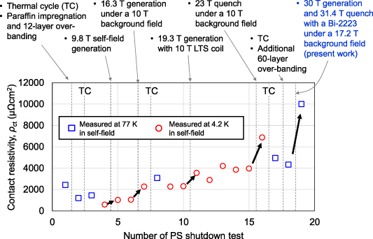
Figure 5. History of experiments on the LNI-REBCO coil and change of the contact resistivity. Each contact resistivity was determined by fitting a simulated field decay curve of an equivalent circuit model to the field decay curve measured in a power supply shutdown test.
Download figure:
Standard image High-resolution image2.3. Set-up for high-field generation test
We installed the LNI-REBCO coil inside the bore of an insulated Bi-2223 coil. These two coils were electrically connected in series. Specifications of the Bi-2223 coil are listed in table 1. As shown in figure 6, the series connected HTS insert was installed in the 130 mm cold bore of the 17 T low-temperature superconductor (LTS) magnet [28] of the Cryogenic Station, National Institute for Materials Science (NIMS). Table 2 shows the inductance matrix of the HTS insert and the LTS magnet. Figure 7 shows a schematic circuit for the high-field generation test. The HTS insert and the LTS magnet were individually charged using two DC power supplies. To precisely observe the LNI-REBCO coil voltage at current holds, we used a highly stabilized DC PS with current stability of 5 ppm h−1 for the HTS insert. Both the LNI-REBCO coil and the Bi-2223 coil was connected to a 1 Ω dump resistor at room temperature. Currents (Ire, Ibi and Ilts) and voltages (Vre-p, Vre, Vre-n and Vbi) were measured as described in figure 7. Three Hall sensors were installed at the top end (Btop), at the centre (Bcen), and at the bottom end (Bbot) of the LNI-REBCO coil along the coil axis as shown in figure 2(b). For a quench detection in the HTS insert, the PS was set to shut down when Vre-p + Vre + Vre-n + Vbi exceeds 0.2 V.
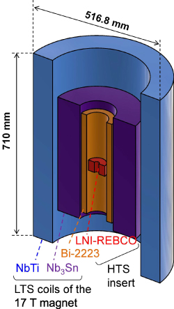
Figure 6. Coil configuration of the high-field generation tests.
Download figure:
Standard image High-resolution image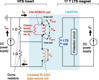
Figure 7. Circuit of the high-field generation tests. The supply current to the LNI-REBCO coil (Ire), that to the Bi-2223 coil (Ibi) and the power supply current for the LTS coils (Ilts) were measured using shunt resistors. For the LNI-REBCO coil, voltages for the terminal conductors (Vre-p and Vre-n; see also figure 2(b)) in addition to the coil voltage (Vre) were measured. For the Bi-2223 coil, the coil voltage (Vbi) was measured.
Download figure:
Standard image High-resolution imageTable 2. Inductance matrix of the HTS insert (REBCO and Bi-2223 coil) and the LTS coil.
| REBCO | Bi-2223 | LTS | |
|---|---|---|---|
| REBCO | 0.048 H | 0.038 H | 0.179 H |
| Bi-2223 | 0.038 H | 0.495 H | 2.77 H |
| LTS | 0.179 H | 2.77 H | 159 H |
Operating parameters at a 30 T central field are listed in table 3. At Ire (≈Ibi) = 265 A, the central field reached 30 T in a background field of 17.2 T generated by the LTS coil. During this operation, Ic of the LNI-REBCO coil was estimated to be 733 A considering field- and field angle-dependencies of the Ic of the REBCO conductor [23]. Note that this estimation did not consider the conductor Ic drop due to the additional over-banding described in figure 4 and therefore the actual coil Ic should be lower than this value. The calculated maximum hoop stress BzJR and the maximum compressive stress are 461 MPa and −16.7 MPa, respectively. Note that these stresses did not consider the effects of winding tension, over-banding, thermal contractions and Lorentz's forces generated by the screening current [8, 29–31].
Table 3. Coil parameters at a 30 T central field.
| Operating parameters | Unit | LNI REBCO coil | Bi-2223 coil | LTS coil |
|---|---|---|---|---|
| Operating current | A | 265 | 241 | |
| Calculated field contribution | T | 9.3 | 4.1 | 17.2 |
| Calculated coil critical current | A | 733 a | 513 | — |
| Calculated max. hoop stress, BzJR | MPa | 461 | 204 | — |
| Calculated max. compressive stress | MPa | −16.7 | −32.7 | — |
a Conductor Ic drop during winding process is not considered.
3. Experimental results
3.1. First charging test: 30 T generation
Figure 8 shows results of the first charging test. The black solid line, the red dashed line, and the blue dashed-dotted line show the central field Bcen, the supply current to the HTS insert Ire (≈Ibi), and the LTS magnet PS current Ilts, respectively. Firstly, we charged the LTS magnet to 241.0 A to generate 17.2 T. We then step-by-step charged the HTS insert with 2–5 A overshooting operations to remove residual voltages generated by relaxation of the screening current. At Ire = 265.6 A, Bcen showed 30.0 T. This value is 2% lower than the calculated field of 30.6 T at 265.6 A, a difference which is mainly due to the effect of screening currents in the LNI-REBCO coil. After holding the coil currents for 15 min, all the coils were discharged without any quench.
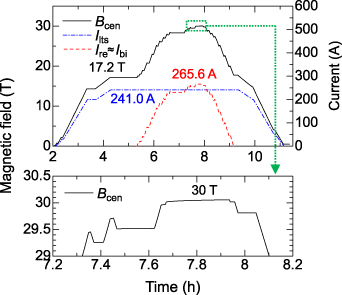
Figure 8. Results of the first charging test: 30 T generation.
Download figure:
Standard image High-resolution imageFigure 9 shows the voltage–current characteristics of Vre (open circle: coil winding), Vre-p (open triangle: soldered part between winding and outer electrode) and Vre-n (open square: soldered part between the winding and inner electrode) in the first charging test to 30 T. Vre does not show normal voltages in the charging and discharging processes. Vre-p shows normal voltage corresponding to 0.5 µΩ in the charging and discharging process. Vre-n shows those to ∼2.3 µΩ during charging and 3.3 µΩ during discharging, which implies that an electromagnetic force progressively delaminated the soldering between the REBCO conductor and the negative (inner) electrode under a high field. Although these results show that the coil winding itself did not degrade during charging/discharging, we need to design a countermeasure to avoid damage to soldered connections. We believe that locating a soldered joint in a low-field region, such as the space above the coil winding, is an effective approach and will employ such an option for future coils.

Figure 9. The voltage–current characteristics of the LNI-REBCO coil voltage Vre, the voltages for the terminal conductors Vre-p and Vre-n (see figure 2(b)) in the first charging test to 30 T. These voltages are averaged values at each current hold after overshooting.
Download figure:
Standard image High-resolution image3.2. Second charging test: quench at 31.4 T
3.2.1. Overview of the test result.
We charged the HTS insert again in the background field of the LTS magnet until a quench occurred in the LNI-REBCO coil. Figure 10 shows Bcen, Ire (≈Ibi) and Ilts traces of the second charging test. The central field reached 31.4 T at Ire = 289.6 A, which corresponds to a conductor current density of 723 A mm−2 and a winding current density of 431 A mm−2. Subsequent events are as follows. (a) Just after reaching 31.4 T, a quench occurred in the LNI-REBCO coil. (b) The DC power supplies for the HTS insert and the LTS magnet detected over-voltages and shut down. (c) The magnetic field generated by the HTS insert decayed in a few seconds. On the other hand, the LTS magnet did not quench and the magnet current was shorted through the cold diode of the protection circuit (see figure 7) and there remained a field of 17.7 T, which is slightly higher than the rated field of 17.2 T, due to an energy transfer from the HTS insert. (d) After the quench event, the LTS magnet was slowly discharged; to extract the energy from the LTS magnet before quenching, we operated the DC PS so as to dump most of the stored energy at room temperature, as seen in figure 10.
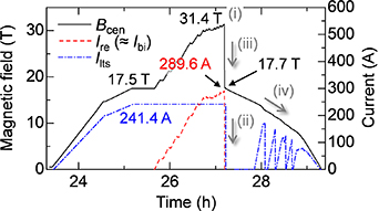
Figure 10. Results of the second charging test with quench of the LNI-REBCO coil at Bcen = 31.4 T.
Download figure:
Standard image High-resolution imageFigure 11 shows the voltage–current characteristics of Vre (open circle), Vre-p (open triangle) and Vre-n (open square) in the second charging test. Vre showed a normal voltage for Ire > 280 A. Vre-n showed the same linear trace with 0.5 µΩ as the first charging test. Vre-p showed a jump at 264.5 A and this produced a Joule heat of 0.55 W just before the quench. We believe that the voltage jump was caused by progressive damage in the soldering; actually, the soldered part was found to be partly delaminated after unwinding the coil.

Figure 11. The voltage–current characteristics of the LNI-REBCO coil voltage Vre, the voltages for terminal conductors Vre-p and Vre-n (see figure 2(b)) in the second charging test with quench at 31.4 T.
Download figure:
Standard image High-resolution imageAfter the test, we warmed up and disassembled the HTS insert to charge the LNI-REBCO coil at 77 K in self-field. The open squares in figure 3 shows the voltage–current characteristic. The plots with Ic = 29.7 A and n = 15 are in good agreement with the plots measured before the quench (the open triangles), which indicates that the coil was protected from the 31.4 T quench.
3.2.2. Transient behaviour during quenching.
Figures 12(a) and (b) respectively show Ire and Vre (solid line), Vre-p (dashed line) and Vre-n (dash-dotted line) just before the 31.4 T quench. The horizontal axes are calibrated such that t = 0 s corresponds to the shutdown of the DC PS for the HTS insert. At t = −23.5 s, we started increasing Ire from 289.4 A with a sweep rate of 0.1 A s−1. Vre showed an inductive voltage of 8.5 mV. At t = −17.5 s, an unexpected rise of Vre was observed. Although we immediately started decreasing Ire, Vre gently increased for 17 s and eventually showed a steep irreversible take-off, i.e. quench. The stable Vre-p and Vre-n values indicates that the quench was initiated from the coil winding. The PS was shut down as Vre-p + Vre + Vre-n + Vbi exceeded the quench detection voltage of 0.2 V.
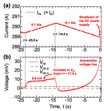
Figure 12. Transient signals just before the quench at 31.4 T. The horizontal axes are calibrated such that t = 0 s corresponds to the shutdown of the DC power supply for the HTS insert. (a) The supply current to the HTS insert Ire (≈Ibi). (b) The LNI-REBCO coil voltage Vre, the voltages for terminal conductors Vre-p and Vre-n (see figure 2(b)).
Download figure:
Standard image High-resolution imageTransient signals during the quench event are plotted in figure 13. Figure 13(a) shows Ire (solid line) and Ibi (dashed line). Figure 13(b) shows Vre (solid line) and Vbi (dashed line). Figure 13(c) shows axial magnetic fields; in order to observe the axial distribution of the magnetic field generated by the LNI-REBCO coil, the normalized axial magnetic fields generated by the LNI-REBCO coil  ,
,  and
and  were calculated from measured Btop, Bcen and Bbot values by the following equations


Figure 13. Transient signals during the quench at 31.4 T. The horizontal axes are calibrated such that t = 0 s corresponds to the shutdown of the DC power supply for the HTS insert. (a) The supply current to the LNI-REBCO coil Ire and the Bi-2223 coil Ibi. (b) The coil voltages of the LNI-REBCO coil Vre and the Bi-2223 coil Vbi. (c) The normalized axial magnetic fields generated by the LNI-REBCO coil at top end  , centre
  and bottom end
  of the LNI-REBCO coil.
Download figure:
Standard image High-resolution imageHere, subscript '*' represents 'top', 'cen' or 'bot'; B* are measured magnetic fields; B*-bi are calculated magnetic fields generated by the Bi-2223 coil; B*-lts are calculated magnetic fields generated by the LTS coil.
After the shutdown of the PS for the HTS insert, Ire and Ibi decreased with different time constants (see figure 13(a)). As shown by figure 13(b), Vre sharply increased and peaked at 58 V at t = 0.8 s. On the other hand, the Bi-2223 coil did not quench because transferred energy from the quenching LNI-REBCO coil to the Bi-2223 coil was so small that it did not exceed the stability margin. Vbi showed a negative inductive voltage induced by the reduction of the LNI-REBCO coil magnetic field and peaked at −62 V. The energy dissipated in the LNI-REBCO coil can be roughly estimated as 8.19 kJ by integrating the products of Ire and Vre during the quench. As a note, the actual dissipated energy should be larger than this value, because Vre included negative inductive voltage. Table 4 shows an energy matrix of the HTS insert just before the quench (Ire = 289.6 A). The table indicates the LNI-REBCO coil dissipated more energy than the self-stored energy, 3.6 kJ; i.e. the LNI-REBCO coil as well dissipated part of the Bi-2223 coil's stored energy.
Table 4. Stored energy matrix of the HTS insert (Ire = Ibi = 289.6 A).
| REBCO | Bi-2223 | |
|---|---|---|
| REBCO | 2.0 kJ | 1.6 kJ |
| Bi-2223 | 1.6 kJ | 20.7 kJ |
| Total | 3.6 kJ | 22.3 kJ |
As shown in figure 13(c),  ,
,  and
and  were in good agreement, which indicates that the magnetic field homogeneously decayed along the axial direction during the quench. This is one of the specific behaviours of the LNI coil [15].
Figure 14(a) shows a comparison between the supply current to the LNI-REBCO coil normalized by the initial value  (=Ire(t)/Ire(0)) and
  .
.  decayed more quickly than
  and this behaviour is caused by a reduction in the circumferential current due to current bypassing through copper sheets. Here, we introduce the current bypass ratio η, defined by the following equation

Figure 14. Transient signals during the quench at 31.4 T. The horizontal axes are calibrated such that t = 0 s corresponds to the shutdown of the DC power supply for the HTS insert. (a) The normalized supply current to the LNI-REBCO coil  and the normalized central magnetic field generated by the LNI-REBCO coil
  . (b) The current bypass ratio η defined by equation (3). The data after t = 3.0 s were deleted after considering the very low signal to noise ratio.
Download figure:
Standard image High-resolution imageThe parameter η gives a rough approximation of the 'current bypassing zone' propagation ratio inside the winding and η = 1 corresponds to full propagation. Figure 14(b) shows the time evolution of η during quenching. Immediately after the quench initiation, η increased and saturated at 0.45, i.e. the current bypassing zone did not fully propagate before the HTS insert was discharged.
4. Discussion
We developed a multi-physics numerical simulation model of the present LNI-REBCO coil in order to analyse the detailed transient behaviour during the quench at 31.4 T. In addition, we investigated factors that contributed to protect the coil from damage.
4.1. Quench simulation model
We constructed a numerical simulation model of the LNI-REBCO coil based on an electrical circuit model in combination with a thermal conduction model. The electrical circuit model considers the magnetic field generated by the Bi-2223 coil and the LTS coil.
Figure 15 shows a schematic of the electrical circuit model, which is based on an equivalent circuit model for the LNI coil [15, 20] and on models for the NI pancake coil [32–34]. Each turn is composed of an inductor (L), the effective resistance of the superconductor (Rsc) and the resistance of the copper stabilizer (Rst). A turn is parallel connected to the resistance of the copper sheet (Rsht) through a contact resistance (Rc). We note that we neglected the contact resistances between axially adjacent turns since the axial contact areas were about 40 times smaller than the radial contact areas. Rsc is described by the following equation
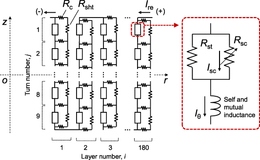
Figure 15. Schematic of the electrical circuit model of the LNI-REBCO coil. Each turn is magnetically coupled to the other turns and the Bi-2223 coil. Rc: contact resistance between conductor and copper sheet. Rsht: resistance of copper sheet. Rsc: effective resistance of superconductor. Rst: resistance of stabilizer. Iθ : current for turn. ISC: current for superconductor.
Download figure:
Standard image High-resolution imageHere, subscript i is layer number and subscript j is turn number in the ith layer. Ec, l, Isc, Ic and n are the electric field criterion (1 µV cm−1), the circumferential length of the turn, the current flowing in the superconducting layer, the critical current and n-index, respectively. The field (B) and field angle (θ) dependency of Ic are represented by a function described in [23]. The temperature (T) dependency of Ic was calculated by the following equation [35, 36]
Here T* is a scaling parameter for the temperature dependence of Ic. We used T* = 19.5 in the present simulation. In addition, the Ic drop distribution, presented in figure 4, was also considered. We obtained a local Ic in the winding by multiplying the Ic drop ratio (see the right vertical axis of figure 4) to the value obtained by equation (5). In addition, based on the voltage–current characteristic measurements of short conductor samples from the LNI-REBCO coil, the n-index for equation (4) was set as 50 for the no Ic drop turns, 16 for most Ic drop turns, and 10 only at the uppermost turn of the 89th layer, which is the lowest Ic turn.
Rc and Rsht shown in figure 15 are expressed by the following equations

In this expression, ρct, w, ρcu and dcu are the contact resistivity between conductor and copper sheet, the width of the conductor, the resistivity of copper and the thickness of the copper sheet, respectively. Here, ρct was set to 10 000 µΩ cm2 which was obtained from the current dump measurements at 77 K in self-field after the 31.4 T quench (see figure 5).
Using Kirchhoff's law, circuit equations of the LNI-REBCO coil are simply expressed as the following equation

The vector { (t)} contains unknown circumferential current for each turn at a time step (t). Matrix [C1] consists of Rsc, Rmt, Rc, Rsht and self and mutual inductance for each turn. Vector {C2} consists of Rc, Rsht, self and mutual inductance for each turn, Ire, circumferential currents at the previous time step
  and inducted voltages by the decay of Bi-2223 coil current.
Figure 16 shows a schematic of the thermal conduction model which assumes a single turn as a thermal element. For simplicity, the heat capacity of the copper/insulation sheets between the layers were combined into each element. Assuming that there is no cooling effect from outside of the coil, the heat balance equation for the element of the jth turn in the ith layer is expressed by the following equation
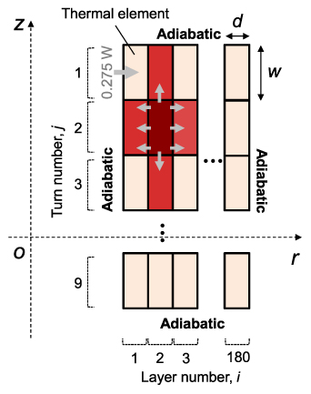
Figure 16. Schematic of the thermal conduction model of the LNI-REBCO coil.
Download figure:
Standard image High-resolution imageIn this equation, t, C, A, gJ, hct and d are respectively time, the combined heat capacity per unit volume, which comprises the heat capacities per unit volume of copper and Hastelloy, the cross-sectional area of the turn (or element), the Joule heat generation in the winding, the heat transfer coefficient between adjacent turns, and the overall thickness of the layer (or element). Here hct was determined based on [37]. While gJ consists of the Joule heating in each turn and those in the facing contact resistance and copper sheet, which were calculated from the current distribution obtained from the electrical circuit model. Considering 0.55 W Joule heating at the soldered part between the winding and the inner electrode, half of this value (0.275 W) was added to the inner-uppermost element.
Solving equations (8) and (9) simultaneously, we analysed the time-varying current distribution and temperature distribution inside the winding. As initial conditions, we set a uniform circumferential current distribution of 289.6 A and a temperature distribution of 4.2 K. Figure 17 shows Ic distribution at the initial state considering magnetic field- and magnetic field angle-dependencies [23] and Ic drop distribution (see figure 4). We assumed that Ire and Ibi start decaying with the waveforms obtained in the experiment, seen in figure 13(a), when the LNI-REBCO coil voltage reaches 0.2 V.
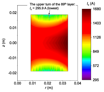
Figure 17. Critical current (Ic) distribution at 31.4 T at 4.2 K assuming a uniform circumferential current distribution of 289.6 A, which considers magnetic field- and magnetic field angle-dependencies on Ic and Ic drop distribution in figure 4.
Download figure:
Standard image High-resolution image4.2. Comparison between simulated results and experimental results
Figures 18(a)–(c) show 
 Vre and η obtained by the simulation. For comparison, the corresponding experimental results in figures 13 and 14 are presented again in figures 18(a')–(c'). The simulated transients are in good agreement with the experimental results. That is, the simulation model well reproduces the quench event. To obtain more accurate results, it may be necessary to take into account the effect of eddy currents induced in the copper sheets, the temperature dependency of ρct, the effect of radial compression on ρct, and the dependency of T* on magnetic field and its angle.

Figure 18. Comparison between simulation results (a)–(c) and experimental results (a')–(c') of transient signals during the 31.4 T quench. (a) and (a') Normalized supply current to the LNI-REBCO coil  , axial magnetic fields at the top end (
 ), at the centre (
 ) and at the bottom end (
 ) generated by the LNI-REBCO coil. (b) and (b') LNI-REBCO coil voltage (Vre). (c) and (c') Current bypass ratio (η) defined by equation (3). The simulation employed ρct = 10 000 µΩ cm2. Experimental results are the duplicates of data in figures 13 and 14.
Download figure:
Standard image High-resolution imageFigures 19(a)–(d) show simulated results of maximum circumferential currents, voltages, maximum temperatures and maximum hoop stresses (BzJR), respectively; each result is plotted per ten layers.
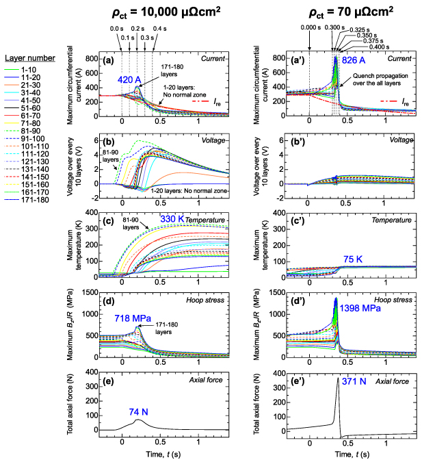
Figure 19. Simulated transient signals during quench at 31.4 T with ρct of 10 000 µΩ cm2 (a)–(e) and 70 µΩ cm2 (a')–(e'). (a) and (a') Maximum circumferential currents. (b) and (b') Voltages. (c) and (c') Maximum temperature. (d) and (d') Maximum hoop stress BzJR. (e) and (e') Summation of axial Lorentz's forces in the winding. Each result is plotted per ten layers. t = 0 s corresponds to the timing when Vre exceeds 0.2 V.
Download figure:
Standard image High-resolution imageFigures 20(a) and 21(a) respectively show the corresponding distributions of circumferential current and temperature over the winding cross-section at t = 0.0 s, 0.1 s, 0.2 s, 0.3 s and 0.4 s. These figures give more details of the quench propagation. Supplementary videos (available online at stacks.iop.org/SUST/34/064003/mmedia) show the sequential transition from t = −0.1 s to 0.4 s of circumferential current (10000_IθDist_-0.1–0.4s_SuST.avi) and temperature (10000_TempDist_-0.1–0.4s_SuST.avi).
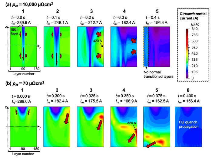
Figure 20. Simulated circumferential current distribution on the cross-section of the LNI-REBCO coil. (a) Results in the case of ρct = 10 000 µΩ cm2 at t = 0.0 s, 0.1 s, 0.2 s, 0.3 s and 0.4 s as indicated in figure 19(a). (b) Results in the case of ρct = 70 µΩ cm2 at t = 0.000 s, 0.300 s, 0.325 s, 0.350 s, 0.375 s and 0.400 s as indicated in figure 19(a'). The sequential transitions for (a) and (b) can be seen in supplementary videos (10000_IθDist_-0.1–0.4s_SuST.avi and 70_IθDist_-0.1–0.4s_SuST.avi, respectively).
Download figure:
Standard image High-resolution image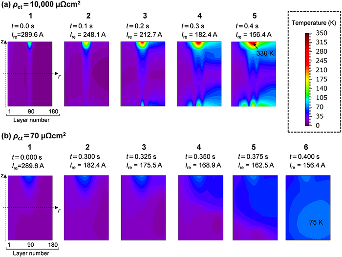
Figure 21. Simulated temperature distribution on the cross-section of the LNI-REBCO coil. (a) Results in the case of ρct = 10 000 µΩ cm2 at t = 0.0 s, 0.1 s, 0.2 s, 0.3 s and 0.4 s as indicated in figure 19(c). (b) Results in the case of ρct = 70 µΩ cm2 at t = 0.000 s, 0.300 s, 0.325 s, 0.350 s, 0.375 s and 0.400 s as indicated in figure 19(c'). The sequential transitions for (a) and (b) can be seen in supplementary videos (10000_TempDist_-0.1–0.4s_SuST.avi and 70_TempDist_-0.1–0.4s_SuST.avi, respectively).
Download figure:
Standard image High-resolution imageAs seen in figure 20(a), the current distribution was nonuniform and rapidly changed with time. This nonuniformity is a particular feature for NI and LNI coils having bypass circuits inside the winding.
As seen in figure 20(a)- 1, the quench started from the uppermost turn of the 89th layer, which was the lowest Ic region seen in figure 17 considering the Ic drop due to the over-banding and the magnetic field dependencies. The temperature of this region had been increasing from 4.2 K by Joule heating at the solder joint between the winding and the inner electrode, which led the coil to quench. The circumferential current distribution shown in figure 20(a) indicates that the circumferential currents of turns in this layer decreased by current bypassing to other turns through the contact resistances and copper sheet. Correspondingly, the voltage over the 81st–90th layers, including the quench initiation turn, started to rise as seen in figure 19(b). This 'current bypassing zone' propagated toward both inner and outer parts of the coil. Normal voltages appeared sequentially in an inner part (21st–80th layers) and the outer part (91st–180th layers). In contrast, the normal voltages did not appear in the innermost part (1st–20th layers), seen in figures 19(b) and 20(a)–5. As a result, the quench progressed with the propagation of the current bypassing zone. Howeve r, it should be noted that not all such zones necessarily transited to the normal state.
As shown in figures 20(a) and 21(a), the current bypassing zone and the temperature rise initially propagated in the axial direction, and then propagated in the radial direction along the top and bottom ends, where the temperature margin of the REBCO conductor is the smallest. The temperature propagation velocity in the axial direction (vz ) was almost constant at 0.0 s < t < 0.4 s and was estimated to be 85 mm s−1. On the other hand, the temperature propagation velocity along the radial direction (vr ) noticeably depends on time domain; it was 10 mm s−1 at 0.0 s < t < 0.12 s and 145 mm s−1 at 0.12 s < t < 0.40 s.
There are two major driving forces for propagation of quenching (i.e. current bypassing): (a) Joule heating due to bypass current through the contact resistances and copper sheets, and (b) electromotive forces induced by the reduction in magnetic flux of quenching turns and by those of the Bi-2223 coil. The former, (a), is the main driving force for the axial quench propagation seen in figures 20(a)–1 and (a)-2. Figure 22(a) shows the distribution of the bypass current through the contact resistances and the copper sheet in the 89th layer at t = 0.0 s. Since the resistance of the copper sheet (Rsht) was two orders of magnitude lower than the contact resistance (Rc), Joule heating generated by current bypassing distributes over the entire layer and it accelerates the axial propagation. The latter, (b), dominates the propagation in the radial direction which is attributed to strong magnetic coupling between turns in the radial direction. Electromotive forces increase the currents of unquenched adjacent turns and make them quenched. In the present experiment, the electromotive force induced by the reduction in the magnetic field generated by the Bi-2223 coil also accelerates this type of propagation for t > 0.12 s since Ibi started to decrease at this time (see figure 13(a)). These driving forces provide a fast quench propagation of an LNI-REBCO coil compared to an ordinary insulated REBCO coil [38].

Figure 22. Simulated distribution of bypass current through the contact resistances and copper sheet in the 89th layer of the LNI-REBCO coil at t = 0.00 s. The red arrows show bypass current through the contact resistances and copper sheet. (a) In the case of ρct = 10 000 µΩ cm2. (b) In the case of ρct = 70 µΩ cm2.
Download figure:
Standard image High-resolution imageAs shown in figure 19(c), the peak of the maximum temperature inside the winding was 330 K, which is lower than a reported temperature causing degradation (>500 K) for a paraffin impregnated REBCO coil [39]. As shown in figure 21(a)- 5, the peak temperature located at the uppermost turn of the 89th layer, which was the quench origin turn. The temperature of the unquenched region was as low as 40 K; i.e. there was a large temperature gradient inside the winding. The peak temperature of 330 K is much lower than the peak temperature, ≫1000 K, estimated by the adiabatic heating model under current discharging mode [14]. This is owing to the fast propagation of quench, or current bypassing zone.
While the current bypassing zone rapidly propagates, additional currents were induced in unquenched turns. Thus the circumferential current peak at 420 A was formed in the unquenched zone of the outermost layer (see figures 19(a) and 20(a)–3), generating a peak hoop stress (BzJR) of 718 MPa (see figure 19(d)). Although this stress is high, it does not exceed the irreversible stresses limit of the REBCO conductor (760 MPa [40] and 800–830 MPa [41]).
As seen in figure 20(a), the circumferential currents are distributed asymmetrically with respect to the central plane of the coil (z = 0 mm). Therefore, an axial net force (Fz ) was generated, due to decentring between the LNI-REBCO coil and the other outer coils [33]. Values of Fz can be obtained by integrating the product of the circumferential current and the radial magnetic field over the entire winding. Figure 19(e) shows the transient behaviour of Fz . The Fz peak was 74 N (7.6 kgf), which was not harmful for the coil.
Consequently, it is demonstrated that the LNI-REBCO coil was protected from damage during quenching at 31.4 T, which is consistent with the experimental results.
4.3. Effects of lower contact resistivity on the quench propagation behaviour
To investigate the effect of the contact resistivity on the quench propagation, we conducted a 31.4 T quench simulation with the ρct value of 70 µΩ cm2, which was typically reported for NI coils [27]. The other parameters were the same as the previous simulation.
Figures 19(a')–(e') respectively show simulated results of maximum circumferential currents, voltages, maximum temperatures, maximum (BzJR) and Fz with ρct = 70 µΩ cm2; note that each result is plotted per ten layers. Figures 20(b) and 21(b) respectively show circumferential current and temperature distributions over the winding at t = 0.000 s, 0.300 s, 0.325 s, 0.350 s, 0.375 s and 0.400 s. Supplementary videos show the sequential transition from t= −0.1 s to 0.4 s of circumferential current (70_IθDist_-0.1–0.4s_SuST.avi) and temperature (70_TempDist_-0.1–0.4s_SuST.avi).
At t = 0.000 s, current bypassing zone and temperature rise were slowly propagating from the uppermost turn of the 89th layer to neighbouring turns (see figure 20(b)-1) in the radial direction. The driving force of this propagation is (a) Joule heating generated by bypass current mentioned earlier. During 0.000 s < t < 0.300 s, vr and vz are estimated to be as low as 5 mm s−1 and 8 mm s−1, respectively, which were close to the velocity reported for the insulated REBCO coil [38]. Figure 22(b) shows the bypass current distribution in the 89th layer at t = 0.000 s. In this case, bypass current was localized since Rct was comparable to Rsht. Therefore, the propagation velocity in the axial direction was low, unlike the case of ρct = 10 000 µΩ cm2. Incidentally, a similar discussion has been published for a NI REBCO pancake using conductive epoxy resin in [42]. The behaviour of a bypass current along the axial direction, which is related to the ratio between Rct and Rsht, as described in figure 22, is similar to the acceleration mechanism of the normal zone propagation velocity of an REBCO conductor with an increased interfacial resistance between the superconducting layer and the stabilizer [43, 44].
At t = 0.300 s, an extremely rapid propagation of current bypassing zone appeared from an upper region in the outermost layer (see figure 20(b)-2); the current bypassing zone spread over the entire coil winding in just 0.1 s as shown in figures 19(a') and 20(b)-2–(b)-6. The driving force of this propagation is (b) electromotive forces induced by reduction in magnetic flux described earlier. While the current bypassing zone rapidly propagated, additional currents were induced in unquenched turns; such current increase is clearly shown in the yellow and red colours part in the gradation images in figures 20(b)-2–(b)-5. This results in the formation of a very high circumferential current peak of 826 A in the 174th layer at t= 0.350 s as seen in figure 19(a') and figure 20(b)-4. The current peak was quickly moving with time from the outer upper region to the inner lower region (see red arrows in figure 20(b)). The phenomenon enormously accelerated propagation of the current bypassing zone, i.e. quench, over the coil winding; this is a notable characteristic nature of the LNI coil having a low contact resistivity. Actually, during 0.300 s < t < 0.400 s, vr and vz are estimated to be 874 mm s−1 and 555 mm s−1, respectively; they are an order of magnitude faster than those for ρct = 10 000 µΩ cm2 and comparable to the quench propagation velocity for LTS coils.
Due to the high propagation velocities, the peak temperature was as low as 75 K (see figure 19(c')), which is four-fold lower than that for ρct = 10 000 µΩ cm2. To the contrary, the current peaks in this case becomes extremely high, resulting in a local hoop stress (BzJR) near the current peak turn that reached 1398 MPa, as seen in figure 19(d'), which is nearly the double of the irreversible stresses of the REBCO conductor, hence causing mechanical damage. Due to the rapid movement of the extremely high hoop stress position across the winding, the coil winding might be mechanically loosened after quench. In addition, the peak Fz was increased to 371 N (37.9 kgf), five times larger than that with ρct = 10 000 µΩ cm2, although it does not seem to be a serious problem.
The simulation results indicate that ρct strongly affects the peak values of electromagnetic stresses and temperature during quenching. Figure 23 shows the peak hoop stress σθ, peak and peak temperature Tpeak during a 31.4 T quench as a function of ρct. We added plots with ρct = 600 µΩ cm2 that was the lowest value obtained for the present LNI-REBCO coil (see figure 5) and ρct = 25 000 µΩ cm2 that was obtained for an LNI-REBCO coil in the previous report [15]. In the case of ρct = 600 µΩ cm2, σθ, peak is higher than the irreversible stress of the REBCO conductor, i.e. the coil will be mechanically damaged. In the case of ρct = 25 000 µΩ cm2, Tpeak is higher than the temperature causing the degradation [39], i.e. the coil will be thermally degraded.

Figure 23. Simulated peak hoop stress σθ, peak and peak temperature Tpeak during a 31.4 T quench as functions of ρct.
Download figure:
Standard image High-resolution image
Figure 23 indicates that there is a specific range of 7000 µΩ cm2< ρct < 20 000 µΩ cm2 in which the coil is not damaged either mechanically or thermally. Note that this range is not general and a particular ρct range will depend on the coil parameters and the si tuation of a quench. In addition, the threshold values here, σpeak < 760 MPa and Tpeak < 500 K, are too high and they have to be set to reasonably low values when designing a protection scheme, e.g. σpeak < 600 MPa and Tpeak < 300 K. In this light, σpeak and Tpeak obtained for the present coil are quite high. In addition, a winding technology to achieve a target ρct is indispensable.
The simulation results are summarized as follows:
- (a)The quench propagation mechanism strongly depends on the value of ρct.
- (b)Figure 23 demonstrates the trade-off between σθ, peak and Tpeak, i.e. a higher ρct provides a higher Tpeak and a lower σθ, peak; lower ρct provides a lower Tpeak and a higher σθ, peak. There is a range of ρct that avoids both mechanical and thermal degradation.
- (c)For the present LNI-REBCO coil at 31.4 T, the high ρct of 10 000 µΩ cm2 coincidentally provided protection from a high hoop stress, although it caused a moderately high local temperature. If the coil had a much lower ρct value, such as 600 µΩ cm2, it would be degraded due to a high hoop stress.
As a side note, we can consider coil behaviours out of the range of figure 23 as follows. When ρct is orders of magnitude higher than the value of 10 000 µΩ cm2, the coil should behave as an insulated coil, resulting in a very high Tpeak and a moderate σθ, peak. When ρct takes a much lower value, which might occur in an solder-impregnated NI/LNI coil, Tpeak should be very low and σθ, peak extremely high. Under such a very fast current transient, there might appear a suppression effect on σθ, peak by an inductive reactance. In addition, a quench detection condition might affect Tpeak and σθ, peak and such investigations will be made in the future.
5. Conclusions
We conducted a high-field generation test using an LNI-REBCO coil connected to an insulated Bi-2223 coil under an background magnetic field of 17.2 T generated by LTS coils. The coils successfully generated a central magnetic field of 31.4 T. Although the LNI-REBCO coil quenched at 31.4 T, this quench did not cause any degradation to the coil. In other words, the LNI-REBCO coil was protected from the quench.
The numerical simulation showed that the peak temperature and the peak hoop stress (BzJR) during the quench were 330 K and 718 MPa, respectively, which are below critical values that cause degradation. The simulation also showed that the contact resistivity of 10 000 µΩ cm2 played an important role to protect the coil. If ρct was as low as 70 µΩ cm2, quench propagation became too fast, inducing large additional currents and a resultant peak hoop stress of 1398 MPa, while the peak temperature was as low as 75 K. In short, the present coil was able to survive thanks to its high ρct of 10 000 µΩ cm2, which suppressed the peak hoop stress at the expense of accepting a higher peak temperature.
For making an appropriate scheme to protect an LNI-REBCO coil from damage, due to overheating and excessive stress during quench, we have to achieve proper processing to implement a target contact resistivity.
Acknowledgments
This work was supported by the JST Mirai-Program Grant No. JPMJMI17A2 and by Grant-in-Aid for JSPS Fellows Grant No. 19J11812. The authors thank Dr T Nagaishi and Mr T Yamaguchi for the measurement of the critical current distribution of the REBCO conductor. The authors also thank members of Cryogenic Station, NIMS for liquid helium supply.
Data availability statement
All data that support the findings of this study are included within the article (and any supplementary files).