
Abstract
A common feature of commercially available conductors based on high-temperature superconducting compounds is the fluctuation of critical current along the length. Fortunately, the practice adopted by manufacturers nowadays is to supply the detailed Ic(x) data with the conductor. Compared to knowing just the average of critical current, this should also allow a much better prediction of the conductor performance. Statistical methods are suitable for this purpose in the case when the fluctuations are regular at the low end of critical current distribution. However, a different approach is necessary at the presence of 'weak spots' that drop out of any statistics. Because of the strong nonlinearity of the current–voltage curve, such a location could transform into a 'hot spot' at transporting direct current (DC), with an abrupt increase of temperature endangering the conductor operation. We present a set of analytical formulas including the prediction of the maximum DC that could be carried sustainably before the thermal runaway appears. It is necessary to know the cooling conditions as well as the properties of the conductor constituents and their architecture. A formula for the voltage appearing on a weak spot, and its dependence on the DC, is also proposed. For this purpose the result of previous theoretical work has been slightly modified after comparing it with numerical iterative computations and finite element modeling. We demonstrate that the derived model allows a powerful analysis of experimental data comprising an estimation of the weak spot parameters i.e. its critical current and the length of the defect zone.
Export citation and abstract BibTeX RIS

Original content from this work may be used under the terms of the Creative Commons Attribution 4.0 license. Any further distribution of this work must maintain attribution to the author(s) and the title of the work, journal citation and DOI.
1. Introduction
Taking advantage of superconductivity as a resistance-less state of some materials requires minimizing any energy impacts that could drive the superconductor into a normal state. Studies of these processes with a particular focus on the coil windings for magnets resulted in the now standard composition of conductor that, along with the functional superconducting material, also contains metallic parts that usually occupy more than 50% of its cross-section [1]. A wealth of research has been dedicated to the development of rules and models for optimal use of such auxiliary materials with regard to the stability of operation, i.e. the tolerance with respect to various disturbances leading to a temperature rise [2–5]. Experimental testing of conductor stability by applying a local heat pulse became a standard methodology for low-temperature superconductor wires and magnets [6–13], and has been transferred to the study of conductors based on high-temperature superconductor (HTS) materials too [13–25]. In some investigations of HTS tapes and coils, the quench was induced by other means like short overcurrent pulse [26], by applying a magnetic tip [27], or by laser irradiation [28].
Normally in these studies, the position where the temperature starts to rise was known a priori. However, in several experiments on HTS magnets, unexpected locations have been detected, leading to the suspicion that a defect at a particular point of the tape causes local overheating [29, 30]. A possible explanation of this observation is a local reduction in the critical current, Ic. It could be the consequence of mechanical damage during coil winding that produces a series of cracks [31–34]. Nevertheless, in the second generation of HTS tapes prepared in form of coated conductors (CCs), a fluctuation of the conductor's critical current has been commonly detected just after its production [35–43]. This phenomenon, nicknamed the 'Ic(x) feature', attracted a lot of interest in the research focused on the development of a resistive fault current limiter (FCL) device [44–48]. Dedicated numerical modeling methods were developed to reproduce all the essential features of the electro-thermal problem in the composite CC tape [40, 49–51]. Also, in the HTS magnet design, the observed volatility in the local critical current attracted growing attention. For example, in the coil stability tests, detailed knowledge of the Ic variability along the conductor length is essential to ensure that the quenching will be initiated by the heater and not in the sections with a low local critical current [52]. Hot spots originating from inhomogeneity have been identified in some cases as the limitation of high-field magnet performance [30, 53–55], and contributed to the conservative design concept, substantially limiting the exploitation of the conductor transport capability [56]. Delivering the information about the Ic(x) distribution together with the supplied tape has become a common practice thanks to the development of scanning techniques [37, 57–59] suitable for long-length reel-to-reel inspection [60–63].
With the help of statistical methods, one can implement the fluctuations of critical current into the design of a superconducting device, provided the conductor properties follow a regular pattern [64–68]. Nevertheless, the focus of this paper is on an 'individual' inhomogeneity like the one shown in figure 1. From all the data provided for the purchased 50 m of tape, only the portion around the lowest value of Ic is shown. In the case of selecting for a short-sample test, for any of the 10 cm long sections marked A, B, C, E a critical current of at least 160 A would be determined. However, there is a location in section D, with the critical current reduced by sim 15%. The properties of this 'weak spot' fall outside of the statistics characterizing the rest of the tape. Fortunately, the supplier's information allows investigation of the electro-thermal process in this location when transporting an electrical current. This is the main topic discussed here. Our analysis is similar to the stability study of HTS coils [69–71]; however, the heated region is not the whole coil winding but only the weak spot and its surroundings. Longitudinal heat flow along the conductor length is considered relevant in the cooling of defects with the length of a few millimeters [72, 73]. On the other hand, we disregard a lateral non-uniformity, and assume that the local heating happens in a strip stretched across the tape width [74–76].

Figure 1. Detail of Ic(x) data of an industrially produced coated conductor tape.
Download figure:
Standard image High-resolution imageOur main concern is illustrated in figure 2, showing the possible scenarios of temperature evolution in the weak spot after switching on the DC, I. For currents up to a certain limit, marked Itr, the temperature would rise for some time, and then attain a stable value. When the supplied current is above Itr, a fast rise of temperature occurs called the 'thermal runaway' [16, 30, 77–79], and the weak spot converts to the 'hot spot' [44, 49, 73, 80, 81]. A reliable prediction of the thermal runaway current, Itr, is therefore of utmost importance. The significance of understanding the transformation from a weak spot to a hot spot for devices operating at liquid nitrogen temperatures is underlined by a very slow to non-existent spread of the normal zone in HTS tapes [14, 50, 63, 82–85], which even led to proposals for changing the tape architecture [86].

Figure 2. Evolution of local temperature in a weak spot at transporting the DC I.
Download figure:
Standard image High-resolution imageThe paper is organized as follows: in section 2, the formulation of the problem we intend to solve i.e. predicting the thermal runaway current for a conductor containing a weak spot with certain characteristics, is presented. In section 3, we first mention a simple iterative numerical procedure allowing us to find the conditions for the thermal runaway that at the same time represent the limits of a stable operation. Then, we show that after some simplifications it is possible to derive the analytical expressions for predicting Itr from known parameters of the weak spot, the conductor architecture, and the cooling conditions. After checking the agreement with the results of the numerical iterative procedure, we examine in section 4 the analytical formula for Itr and discuss the impact of various parameters on the conductor stability. Then, in section 5 we present the verification of our previous findings by measurements. Experimental identification of a thermal runaway is rather challenging. Fortunately, we have found a way to widen the range of the analyzed current-voltage data adopting the formula proposed in [70] in a slightly altered form. This empirical modification provided results in excellent agreement with two numerical procedures: in addition to the numerical iterative solution of the heat balance, we have utilized a finite element code to model the process of hot spot creation. As a result, we can now propose an analytical expression capable of predicting the current-voltage curve when approaching Itr in a quasi-static DC test. By using this procedure of analyzing experimental data we have found that the power-law approximation of the current-voltage curve measured on the sample containing a weak spot is distorted due to the elevation of temperature that is varying for each data point. The finite element computation, in which a realistic composite architecture as well as the heat transfer characteristic including the hysteresis at critical heat flux was implemented, gave identical results.
The theory presented here is not limited strictly to the second generation of HTS conductors; however, several examples will be presented having in mind a CC tape. We will refer to two hypothetical CC tapes (see table 1) based on the rare-earth superconducting compound REBCO (where RE represents a Rare Earth element like Y, Sm, Eu, Gd,... and B replaces Ba, C replaces Cu and O stands for oxygen) with the properties essential for the stability shown in table 1. The calculation of thermal conductivity is described in detail in section 3, formula (16). The specific heat is obtained by summing up the heat capacities of all the tape layers. Properties of materials at 77 K used in these calculations are reported in the appendix. The Tape MAG resembles the standard tape utilized for coil winding [87] and Tape FCL has the characteristics dedicated for the use in a resistive FCL [88]. We disregard the possibility of current transfer to parallel metallic paths [89, 90], which nevertheless could push thermal runaway to higher currents for some conductors or operating conditions.
Table 1. Architecture and some thermal properties at 77 K of two hypothetical tapes used in the illustrative computations presented throughout this paper.
| Tape MAG | Tape FCL | |
|---|---|---|
| Tape width, wT (mm) | 4 | 12 |
| Hastelloy (µm) | 50 | 100 |
| REBCO (µm) | 1 | 3 |
| Ag (µm) | 4 | 2 |
| Cu (µm) | 40 | 0 |
| Longitudinal thermal conductivity (W K−1 m−1) | 242 | 16.8 |
| Specific heat of 1 m of tape (J K−1 m−1) | 1.62 | 1.91 |
Table 2. Thermal conductivity and specific heat of materials used in this paper.
| Material | Thermal conductivity at 77 K (W K−1 m−1) | Specific heat at 77 K (J K−1 cm−3) |
|---|---|---|
| Hastelloy | 7.75 | 1.53 |
| REBCO | 8.8 | 1 |
| Ag | 479 | 1.72 |
| Cu | 517 | 1.75 |
In our considerations, we deal with only one single weak spot in an otherwise 'healthy' tape. In the case of a number of hot spots in a long conductor, this could seem to be an exaggeration. However, due to a highly nonlinear current–voltage curve of HTS material, after the starting of thermal runaway in one place, the rest of the conductor carrying the same current will not reach the runaway temperature. Thus, there is always one particular location relevant to the stability examination. Not surprisingly it is the value of critical current in the weak spot that is essential for predicting Itr. Nonetheless, our analysis reveals the role of other factors, in particular, the defect dimension. In the applications where the tape is exposed to a magnetic field with a varying strength like electromagnets, the original low-field Tapestar data should be modified accordingly. This would probably re-order the expected Itr ranking, and shift attention to the locations experiencing the maximum magnetic field. However, also in large coils, the thermal runaway will start in a weak spot with the lowest Itr, and the other weak spots (with higher Itr) will still be in the conditions of a stable temperature.
2. Formulation of the problem
The problem to solve is schematically illustrated in figure 3. A superconductor wire carrying DC electrical current, I, exhibits the following property: critical current is Ic0 everywhere except the location with the length Δxws where it is reduced to Icmin. This is the 'weak spot' in which an appreciable electric field Ews would appear, while the rest of the conductor remained resistance-less at Ic0 > I > Icmin. As a consequence, the local power dissipation  will start. We focus here on investigating a small-scale non-uniformity with Δxws in the millimeter range [37, 42, 73]. Then, the weak spot temperature, Tws, can be considered uniform in the whole volume of the conductor within Δxws. Such simplification, essential for the development of an analytical model, differs from the formulation used in numerical modeling where the composite structure has been implemented [27, 41, 73, 80, 91, 92]. The local rise of temperature triggers a heat flow towards the ambient, while the latter is assumed to keep the baseline temperature T0 all the time. The expression controlling the heating process is

Figure 3. Approximation of weak spot used in theoretical modeling.
Download figure:
Standard image High-resolution imagewith Cws being the heat capacity of the weak spot (J K−1), and Pcool the power of heat removal [W]. At the ambient temperature T0 one could expect in the first approximation that

where Kws is the thermal conductance [93] between the weak spot and its ambient [W K−1]. The basic arrangement we have in mind here is the HTS wire immersed in liquid nitrogen with T0 = 77.3 K. We also assume that the rest of the conductor, where the critical current is equal to Ic0, is kept at T0. In order to allow a variation of cooling efficiency with temperature, we introduced the linear approximation

with K0 , K1 derived from the wire geometry, its thermal properties, and the cooling conditions. The method of estimating these parameters will be described in more detail later.
Taking into account that the REBCO layers in CC tapes carry >1010 A m−2, at electric fields in the 10−4–10−2 V m−1 range there will be no significant flow of current in parallel metallic layers of the CC tape at 77 K, in contrast to the studies exploring current sharing [41, 94, 95]. Current–voltage characteristic of the weak spot in our analysis is therefore controlled by the intrinsic properties of the superconductor. From the possible approximations [96] we have chosen the power-law
where Ec is the critical current criterion usually taken as 10−4 V m−1, and the exponent n ≫ 1. Further, we assume that the critical current at the weak spot changes with temperature as
i.e. decreasing from the value Icmin at T0 to vanish completely at the temperature Tc. Disregarding a possible variation of n with temperature is another simplification we adopted similarly to some other studies [80, 97–99]. Inserting the relations (2–5) into (1) results in the basic equation analyzed further in this paper
Here, ΔTc = Tc −T0, the auxiliary variable characterizing the weak spot warming is ΔT = Tws −T0, and
is the dissipation at the conditions when the weak spot temperature is equal to the coolant temperature, T0. This happens for the instant of switching the current I on.
The weak spot temperature tends to rise because of the first term in square brackets in (6). Warming of the weak spot, resulting in the ΔT growth, will turn on the cooling power given by the two remaining terms. As we can see, the expression (6) is an equation for variable ΔT with all the remaining quantities being constants. The main concern is that the weak spot temperature remains stable i.e. both sides of (6) are equal to zero. Then, the dissipation term is to be exactly balanced by the cooling terms:
This is illustrated in figure 4, where the dependence of both sides on ΔT at three DC currents is plotted as calculated for a weak spot in the tape with Tape MAG architecture. It is immersed in a liquid nitrogen bath with the thermal conductance parameters K0 = 0.03664 W K−1 and K1 = 0.0002 W K−2 obtained from the considerations explained in the following section.
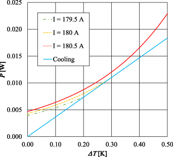
Figure 4. Comparison of cooling power (full line) with dissipation at three values of DC transported by the Tape MAG containing the weak spot characterized by Δxws= 1 mm, Icmin= 150 A, Tc = 87 K, n = 30. The variable on the horizontal axis is the difference ΔT = Tws –T0.
Download figure:
Standard image High-resolution imageIn analogy to figure 2, there are two possible scenarios: at currents up to I= 180 A, which in this case is the value of thermal runaway current, Itr, the solution of (8) exists, resulting in a stable temperature elevated by ΔT over the ambient temperature T0. At higher currents, the increase of dissipation with temperature is too sharp to achieve a solution, and the weak spot temperature starts to grow without a limitation.
What could then happen if the existence of a weak spot had remained undetected because the critical current was established by testing the sample from a 'healthy' portion of the tape? Let us imagine the case when Ic0 = 181 A; thus, the weak spot in our example represents a local reduction of critical current by sim 17%. Supplying such 'nominal' critical current will transform the weak spot into a hot spot exposing the conductor to serious danger of irreparable local damage. Therefore, if one knows that there have been weak spots revealed e.g. in the reel-to-reel procedure [100], it is important to estimate the value of Itr, and take it into account during further considerations. This is the topic of the next section.
3. Triggering of a thermal runaway
In order to identify the maximum value of current, below which the thermal runaway will not occur, we adopted an iterative numerical procedure [68, 69, 101] solving the nonlinear equation (8): here, testing the evolution with the temperature of both sides for different values of the transported current I allows us to find Itr. In the same computation, one also finds the maximum achievable stable temperature of the weak spot, Ttr, fulfilling the condition
where ΔTtr = Ttr −T0.
The outcome of such a numerical procedure is rather straightforward. But, for understanding the influence of various conductors and cooling parameters, the possibility of finding Itr and ΔTtr from (9) in the form of an analytical expression would be helpful. Fortunately, this can be achieved taking into consideration that not only must the two sides of (9) be equal, but also the derivatives with respect to ΔT [69, 70]. In other words, at the intersection of the dissipation curve plotted for Itr and the cooling curve in figure 4, we also observe that the slopes of these two curves are identical. This allows us to articulate the second equivalence
Combining the expressions (9) and (10) leads to a quadratic equation for the unknown ΔTtr:
It has the solution
in which the auxiliary variable is
As we can see, the properties of superconducting material with repercussions on ΔTtr are the n-value and the separation of temperature at which, according to (5), the supercurrents vanish, Tc, from the ambient temperature T0. Surprisingly, the property defining the weak spot, namely its critical current Icmin that is lower with respect to the rest of the conductors, does not play any role in predicting ΔTtr.
In many practical situations, including CC tape operating in liquid nitrogen, the variation of the thermal conductance with temperature is rather weak, and one will find that Δ ≪ 1. Then, with the help of approximating  where
where  , the simplified expression can be derived:
In the case of disregarding the dependence of the thermal conductance on temperature, the K1 term would be zero, and the formula (14) will attain the form identical to the prediction derived in [70] dealing with a coil made from a uniform conductor. It would simply state that a lower n, as well as the operating temperature providing a sufficient reserve with respect to Tc, are the main factors for lowering the probability of a thermal runaway. Thus, if the weak spot is caused by an imperfection in the superconductor microstructure resulting in a reduced critical temperature or weaker flux pinning [42, 102], the thermal runaway would appear sooner. However, improvements in the industrial production of CCs make macroscopic geometrical defects probable causes of weak spots. Therefore, here we undertake the alternative that the superconducting material itself keeps the undisturbed values of Tc and n and the reduction of local critical current from Ic0 to Icmin is due to constrictions in the path available for the flow of current [32, 62, 103–105].
The second term in square brackets in (14) is an improvement with respect to the previous studies on the stability of the superconducting conductors and magnets where the hot spot was determined by local electromagnetic fields interacting with a uniform conductor. For demonstrating how the weak spot parameters Icmin and Δxws influence the thermal runaway and hot spot creation, we must first analyze the role of parameters controlling the heat exchange between the conductor and its environment. The heat removal along the conductor's length to the portions kept at the ambient temperature, T0, should be analyzed separately from the heat flow in a direction transversal to its surface (still at T0). This is schematically indicated in figure 3 by the symbols Q|| and Q⊥, respectively.
Numerous studies of cooling revealed that the efficiency of heat exchange between a heated object and its environment is controlled by a rather complex mechanism of heat transfer in liquid [89, 106–110] and strongly influenced by other factors like the object shape and orientation [111–113] and its surface [114–117]. A rigorous treatment of the subject goes beyond the scope of this work. For practical reasons, we assume that, in the limited range of temperatures relevant for the present analysis, the transversal heat removal from the weak spot surface (in Watt) at the temperature difference ΔT = Tws −T0 can be expressed as

Here, for the cooled surface of the weak spot, we took the product 2wTΔx; i.e. the tape is wetted on both flat faces ignoring the side edges. Also, the temperature in the weak spot is considered uniform across the tape width, wT, as well as its thickness, tT. Regarding the heat transfer coefficient, h0, one can find rather wide-ranging data in the literature, from 100 to 2000 W m−2 K−1 [22, 27, 118, 119]. The linear term, h1, is the first approximation of more complex dependences suggested in the dedicated heat transfer studies [112, 120]. In our experiments, for the Tape FCL suspended in liquid nitrogen, we have found the values of h0 = 350 W m−2 K−1 and h1 = 25 W m−2 K−2. When the same tape was attached to a plate from machinable aluminum nitride (that is commercially supplied under the abbreviation BNP), a better heat transfer was observed, characterized by h0 = 900 W m−2 K−1 and h1 = 50 W m−2 K−2. Throughout the rest of the paper we refer to these two sets of parameters as characterizing the 'standard' and the 'enhanced' cooling in liquid nitrogen bath, respectively.
The tape property that controls the longitudinal heat transfer, Q||, is the tape's (longitudinal) thermal conductivity. It is calculated from the thermal conductivity ki
and the geometry (thickness of the ith layer is ti
,  ) of its constituents:
The longitudinal heat transfer from the weak spot [in Watt] is governed by the equation
in which the temperature gradient would be, in reality, rather complex because a transversal escape of heat influences the longitudinal heat flow. Smart simplification is achieved by using the concept of 'thermal length' expressed by the formula [4, 70]

allowing us to estimate that
i.e. the quantity ΔT = Tws −T0 is again controlling the heat transfer. Using this approximation in (17), and taking into account that from the weak spot location the heat flows in both +x and −x directions, leads to the final formula
Now, we can combine the expressions (15) and (20) to find the total cooling power Pcool = Q⊥ + Q|| , and derive the formulas for two parameters controlling the heat removal that were previously introduced in (3):

It is worth noticing that the only property of the weak spot entering these expressions is its length, Δxws. This is consistent with the comment below the original Ttr formula (12) that the local critical current Icmin does not affect the maximum stable temperature.
It is no surprise that the heat removal along the tape length plays a significant role for short defects, because at Δxws → 0 only the second term in the bracket of (21) survives. In contrast, for long defects with the dimension  , the transversal heat flow through the surface is essential. This is illustrated in figure 5 where the dependence of K0 and K1, respectively, on the weak spot length in Tape FCL is compared for two cooling regimes; the standard and the enhanced one.

Figure 5. Example of thermal conductance coefficients K0 (full lines, axis on the left) and K1 (dashed lines, axis on the right) computed for Tape FCL in two different cooling regimes: standard cooling by liquid nitrogen bath of freely suspended tape (open symbols), and enhanced cooling due to tape touching from one side a ceramic BNP plate with good thermal conductivity (full symbols).
Download figure:
Standard image High-resolution imageWith the K0 and K1 known, we can now calculate the thermal runaway temperature Ttr that at the same time is the maximum temperature at which the weak spot remains stable. Let us find K0 and K1 for various weak spot lengths Δxws in the Tape FCL immersed in liquid nitrogen, and then with the help of (21) and (22) compute the maximum allowed weak spot temperature, either using the formula (12) directly or in its simplified version (14). The result is shown in figure 6 in terms of the difference ΔTtr = Ttr −T0 together with several data points obtained by the iterative numerical procedure. As we can see, the analytical expression (12) agrees perfectly with the results of much more time-consuming numerical computation. The simplified expression (14) overestimates the exact solution, but this difference is negligible for short defects and does not exceed 0.2 mK for long defects. In the same plot the limiting cases of Δxws→ 0 and Δxws → ∞, respectively, are also indicated. Notice that the variation of ΔTtr due to the spot length is the result of including the longitudinal heat removal into our considerations. Still, in the whole range presented, the observed span of ΔTtr is 5 mK only.

Figure 6. Weak spot temperature elevation with respect to the ambient temperature, triggering thermal runaway, ΔTtr = Ttr −T0, as predicted by the exact and simplified formulas (lines) and from the numerical iterative computation (empty symbols) for weak spots of various lengths in Tape FCL. Tc = 87 K, n= 35, cooling in standard conditions characterized by h0 = 350 W m−2 K−1 and h1 = 25 W m−2 K−2. The noticeable point is the rather narrow range of values on the vertical axis limited by two theoretical predictions for the short and long weak spot.
Download figure:
Standard image High-resolution imageOnce we know the value of ΔTtr it is possible to calculate the maximum dissipation in the weak spot at starting thermal runaway:

An exact solution requires inserting ΔTtr here from (12). In pursuit of understanding the influence of various parameters, we have simplified (23) in the following way: because usually K1ΔTtr ≪ K0, it is thinkable to neglect the second right-hand term in (23). Then, using (14) results in the approximation
which could be further simplified for the same reason to the form
The validity of these approximations can be judged from figure 7, where the three expressions are plotted together with the results of the numerical iterative computation. All three curves converge to the same value at Δxws → 0. This is not surprising, because we assumed that in the limited interval of temperatures coming into consideration the thermal conductivities can be taken as constant. Notice that the critical current at the weak spot, Icmin, has again no influence on the local dissipation power at the thermal runaway, Ptr.

Figure 7. Dissipation in the weak spots of various lengths but with the same Icmin= 450 A in Tape FCL, predicted by exact and simplified formulas (lines) and from numerical iterative computation (empty symbols). Tc = 87 K, n= 35, cooling in standard conditions characterized by h0 = 350 W m−2 K−1 and h1 = 25 W m−2 K−2. Negligible difference and fair reproducing of numerical results justifies using simplified expression in further analysis.
Download figure:
Standard image High-resolution imageNow coming to the testing with DC I, the power Ptr is the result of the temperature rise that started at the same current but at temperature T0. By comparing (23) and (9), we can find that the starting dissipation is
On the other hand, it is also
Here, we remember that Icmin is the weak spot critical current established at temperature T0. Then, by combining these two expressions, one can find that the ratio between the thermal runaway current and Icmin is
where we have introduced the auxiliary parameter as
Now, finally the weak spot critical current Icmin enters into the game because the thermal runaway will happen at transporting the current Itr that is proportional to Icmin with the correcting factor on the right-hand side of (28) that, due to the power 1/(n + 1), is not very different from 1. Then, the expressions (28) and (29) provide the most important prediction for the operation and testing of the conductor with known distribution of the weak spots: the tolerable value of current is limited by the weak spot that, to a great extent, is distinguished by the lowest Icmin. This justifies the approach of some tape manufacturers that also report, together with the average and standard deviation of Ic(x) data, the information about the minimum Ic.
It would be nice to have a more explicit expression showing the relevance of various parameters in (29). Therefore, we have examined what happens when taking the more simplified version of (14) which is  . Then, one can find that
where the base of natural logarithms, e, is the approximation of the term  for n ≫ 1. Taking into consideration that K1ΔTtr ≪ K0, further allows us to simplify this expression to the form
Surprisingly the prediction of Itr with this simplified formula is nearly identical with the result of using the exact expression (29), as demonstrated in figure 8. Longitudinal heat flow helps small weak spots to avoid the thermal runaway; therefore, at Δxws → 0, the value of Itr/Icmin would grow to infinity. Asymptotic value for a long weak spot, that can be obtained in the limit Δxws → ∞ in (21), is presented as well. The important point here is that the simplified prediction (31) is in excellent agreement with the results of iterative computations. Thus, instead of solving the problem formulated by equation (6) by numerical means, there is a rather simple analytical expression available for estimating the DC at which the thermal runaway would be triggered:

Figure 8. Thermal runaway current computed for weak spots of various lengths with the same Icmin = 450 A in Tape FCL, predicted by an exact formula (full line) compared with the result of numerical iterative computation (empty symbols) and prediction of a simplified formula (crosses). The weak spot and cooling parameters are the same as in figure 7. Differences cannot be seen with the current resolution.
Download figure:
Standard image High-resolution imageThus, the main factor here is the local critical current Icmin which is the proportionality factor in (32). The rest of the parameters affect Itr much less, due to the exponent 1/(n+ 1): As one can see, reducing the power-law exponent, n, and the defect dimension, Δxws, would push Itr up. A positive effect could be also achieved by an increase in the numerator. This means a better cooling—characterized by the constant term of thermal conductance, K0—as well as a bigger gap between the operating temperature, and the temperature signaling the complete loss of critical current, ΔTc = Tc −T0.
Traditionally, the critical current defined by the 1 µV cm−1 criterion is considered a safe level of current that should be used in short sample testing. Imagine now, as an example, that the weak spot with Icmin = 450 A is located in the conductor which, outside that location, exhibits the critical current Ic0 = 530 A. Then, Ic0/Icmin = 1.18 i.e. the weak spot represents a 15% local reduction of the critical current. An attempt to check the 'undisturbed' value of the conductor critical current Ic0 in an experiment on a sample containing such a weak spot will most probably be hindered by the thermal runaway, as we can see in figure 8 for nearly all the considered weak spot dimensions it will transform into a hot spot at I = Ic0 = 1.18Icmin.
It is reassuring that the predictions presented in figures 6–8, respectively, show that the analytical expressions for the thermal runaway temperature (14) and the power (24), as well as the maximum current transportable before entering the thermal runaway (32), are in excellent agreement with the results obtained by the iterative numerical computations. We take advantage of having at our disposal these analytical expressions in the following section.
4. Factors influencing the runaway current
The practical importance of predicting the current at which the weak spot would convert to a hot spot motivated us to discuss how various tape properties influence the thermal runaway current, by analyzing the formula (32) in more detail. As an illustration in figure 9, we have summarized the data computed for a 3 mm long weak spot. In a wide range of the considered weak-spot critical currents, the quotient Itr/Icmin remains rather comparable even for tapes with rather diverse architectures subjected to different cooling regimes.
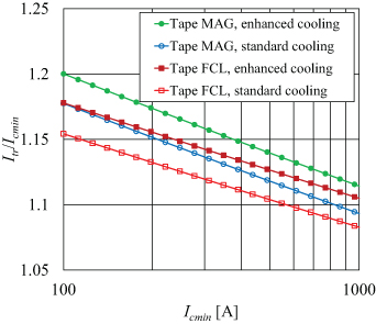
Figure 9. Ratio of thermal runaway current to the critical current in a 3 mm long weak spot in two CC tapes with a different architecture, computed for two different cooling conditions in liquid nitrogen mentioned in figure 5. It is considered that n = 30 for Tape MAG and n = 35 for Tape FCL.
Download figure:
Standard image High-resolution imageThe curves presented in figure 9 exhibit different slopes for two tapes because we considered n= 30 for Tape MAG and n= 35 for Tape FCL. As mentioned already, a lower power n in the current–voltage dependence (4) results in a higher Itr. This is illustrated in figure 10 presenting the data computed for Tape MAG with a 3 mm long weak spot at the standard cooling conditions. Nevertheless, for commercially produced conductors, the higher n is considered a sign of strong and uniform pinning properties of the superconducting layer. Therefore, raising Itr by lowering n artificially is probably out of the discussion. Producers also struggle to advance the temperature Tc in (5) towards the critical temperature of the utilized REBCO compound. Success in such development may have a positive albeit marginal effect on Itr.

Figure 10. Influence on the steepness of the superconductor's current–voltage characteristics on the ratio of thermal runaway current to the critical current in a weak spot. Predictions were computed from (32) for the standard cooling conditions in liquid nitrogen and various exponents n of the power law (4) assuming a 3 mm long weak spot in the Tape MAG.
Download figure:
Standard image High-resolution imageIn the illustrations of our theory presented here, we typically consider a short piece of an HTS tape immersed in liquid nitrogen. Now, we briefly discuss if the prediction (32) could also be useful in the assessment of an HTS coil operating at low temperature (4 or 20 K) achieved by a cryocooler or in a liquid helium bath. First of all, the Icmin values should be taken at respecting such conditions. Let us suppose that the weak spot is caused by an obstacle for the flow of current in the superconductor. Then, we can modify the Tapestar data with the help of the temperature and field dependence obtained on the short sample(s) of the tape, and eventually identify the absolute minimum of Icmin in the whole coil winding at the operating conditions. A clear advantage of low temperatures is in the increase of ΔTc. Regarding the thermal conductance coefficient, K0, this could be rather different in conditions of heat transfer in a 3D object. Interestingly, for the HTS coil operating at 20 K in [69], the value of 0.34 W K−1 was found which is not very far from those illustrated in figure 5. Rather contradictory would be the effect of low temperature and magnetic field on the power law exponent n. The expected increase at lower temperatures could be outweighed by applying a (high) magnetic field. However, because all the parameters (ΔTc, K0, n) appear modified by the power 1/(n+ 1), we do not expect a substantial difference from the conclusions derived, keeping in mind the liquid nitrogen bath and the self-field conditions.
One could have already noticed in figure 8 that the length of a weak spot, Δxws, plays an important role. It appears in the right-hand term of (32) explicitly in the denominator but it is also implicitly involved in K0 through (21). Then, the relevant parameter is the ratio K0 /Δxws, that taking into account (18) can be found in the form
where the thermal length, lth, is defined by (18). This quantity controls the character of the Itr/Icmin dependence on Δxws, dividing the Δxws range into an interval of short defects smaller than lth where the rapid change of Itr/Icmin is observed, and an interval of long defects where Itr/Icmin approaches a roughly constant value. It is illustrated in figure 11, where in the same plot the curves computed for two tapes and two different cooling conditions are presented. For each of the dependences the calculated value of lth is indicated by a vertical arrow. From (33) it is easy to comprehend the rapid growth of Itr/Icmin at shortening the weak spot below lth, and its divergence when approaching Δxws → 0 observed in the graph. It is also understandable that for the long defects i.e. with Δxws ≫ lth this expression tends towards a constant value K0/Δxws ≈ 2wT h0, resulting eventually in the saturation of the Itr/Icmin ratio. It also allows us to find the 'secure' estimate of thermal runaway current for the weak spot with known critical current Icmin, but unknown dimensions, as
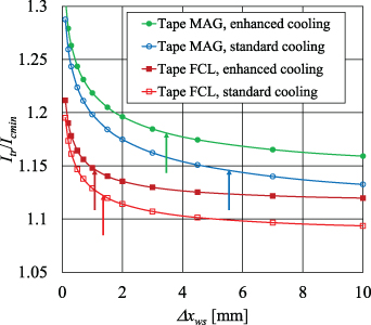
Figure 11. The Itr/Icmin ratio computed for the weak spots of different lengths in two tapes of different architecture. We have considered that Icmin= 150 A and n= 30 in the 4 mm wide Tape MAG while Icmin = 450 A and n = 35 in the 12 mm wide Tape FCL, respectively. Results obtained for standard and enhanced cooling conditions are compared. Vertical arrows indicate the thermal lengths calculated from (18) for each of the curves.
Download figure:
Standard image High-resolution imageFigure 11 nicely illustrates that adding the stabilizing Cu layer enhances the Itr/Icmin ratio [121–123]: it is the additional heat conduction along such a metallic sheath that causes higher thermal conductance resulting in a larger thermal length lth. Then, for example, a weak spot with a dimension of 2 mm is considered 'long' in the Tape FCL but 'short' in the Tape MAG. A similar influence is expected also when adding a non-metallic cover layer, provided it has good thermal conductivity [124, 125].
The plots in figure 11 also give an idea of how much larger currents could withstand short weak spots compared to this conservative estimate: up to sim 10% in the weakly stabilized Tape FCL and up to sim 25% in the Tape MAG with standard Cu stabilization. Probably the most significant finding of this analysis is that at a rather significant difference in the tape architecture the ratio Itr/Icmin has been changed by less than 10%.
5. Experimental verification
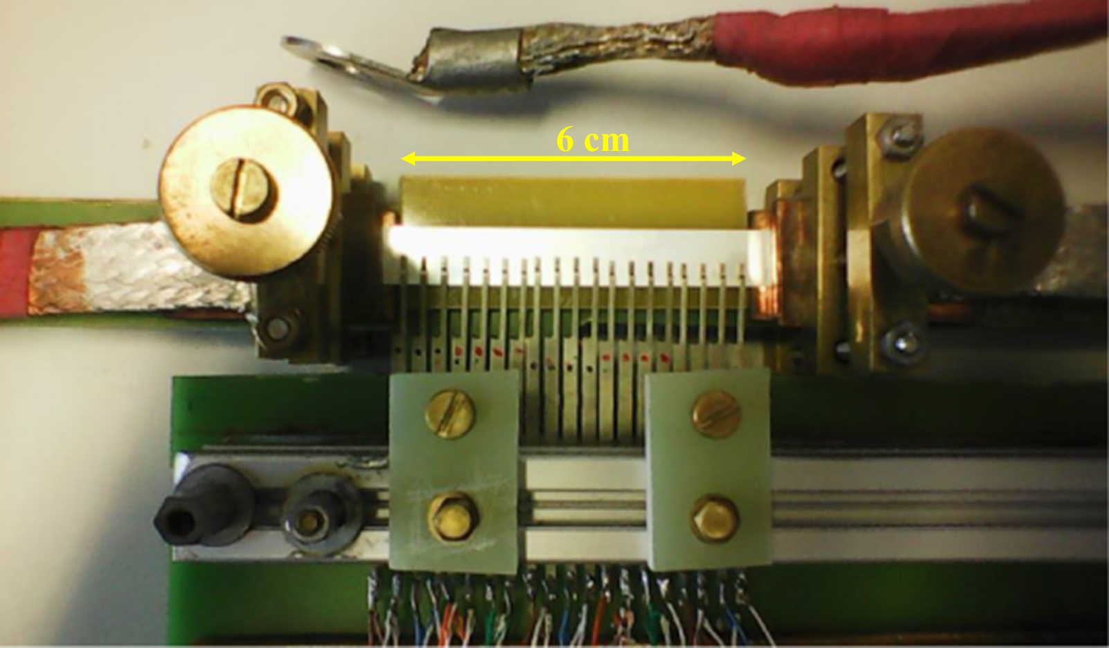
We have tested the validity of formulas predicting the thermal runaway conditions on a series of samples cut from the 12 mm wide tape from recent production [88] that exhibits an impressive critical current close to 800 A, and its architecture is identical with the Tape FCL. We knew from the Tapestar data that up to sim 10% dropouts of critical current are to be expected randomly distributed among the samples. Taking into consideration the studies showing that local defects can be induced in HTS conductors by mechanical stress [31–34, 126] we attempted to create additional, more prominent, weak spots by bending the tape by hand to a diameter as low as 20 mm. Indeed, the existence of weak spots with a wide range of critical currents was confirmed in DC transport tests when the electric field distribution along the sample was recorded with the help of the multitap device shown in figure 12. There are 19 flexible reed contacts, separated by sim 3 mm, touching the sample surface gently and connected by the electrical wiring to the input of a multichannel DC voltmeter. Pressing contacts commonly exhibit larger noise compared to the soldered voltage taps, but for our investigation, it is crucial to minimize a possible modification of local cooling conditions. From the total sample length of 100 mm, the current terminations occupied 20 mm each, leaving the central sim 60 mm part for examination. The experiment was performed in two steps, and in each of them the DC was raised under manual control: first, at a continuous current ramp, the location of the weak spot was identified by noticing the pair of contacts showing the first appearance of an electrical signal from sim 0.2 µV of background noise. The position of the 'active' pair of contacts was fully reproducible but individual for each of the samples. Only this signal was registered in the subsequent step when the current ramp was repeated with small increments, always waiting for the voltage stabilization that we considered a sign of reaching the thermal equilibrium. Eventually, at some value of current, the voltage signal continued to rise—with a growing rate—also at a constant current. At this point, we cut the current in order to avoid damaging the sample. In some cases, we noticed in the subsequent test that a reduction of the critical current or even its complete loss occurred.

Figure 12. Multitap device used for identifying the weak spot locations in CC tapes.
Download figure:
Standard image High-resolution imageFollowing this procedure, we were able to record for each of the samples tested the voltage just on the weak spot with the lowest Icmin. These are then the data we used in comparison with the theoretical predictions. The voltage signal, Utr, detected on the weak spot [127] at the moment of starting thermal runaway fulfills the condition Ptr = Utr Itr. Thus, its value can be determined with the help of (25) and (28) as
Then, both the parameters characterizing the local weak spot, Δxws and Icmin, respectively, have an impact. In figure 13 the set of Utr(Itr) dependences computed using (28) and (35) at a standard cooling regime for three hypothesised values of Δxws = 0.7, 1.4 and 2.3 mm, respectively, assuming n= 25 and Icmin ranging from 100 to 1000 A, is plotted. In the same plot the current–voltage curves measured on the weak spot locations in five samples at the same cooling conditions i.e. immersed in liquid nitrogen and suspended only by current terminations, are inserted. As one can observe only in one case (the tape having the weak spot with sim 600 A of critical current), several points have been caught during the phase of a rapid voltage growth, too. However, in this experiment, the sample was damaged irreparably, and therefore in other trials, we did break the current at an earlier stage of recognizing a rapid signal growth.

Figure 13. Theoretical predictions (curves) for the voltage appearing at the starting thermal runaway computed for three different weak spot lengths in Tape FCL. These are compared with the current–voltage curves measured in standard cooling conditions on the weak spots with various Icmin detected in five different samples (symbols—empty squares). One can notice that the measured curves enter an instability at the voltage levels in, roughly, an inverse proportion to the critical currents, in agreement with the expectation deduced from the expression (35).
Download figure:
Standard image High-resolution imageIt is then rather problematic to define an exact criterion for identifying the thermal runaway in the recorded voltage in a reproducible way. As predicted by (35), the value of Utr is inversely proportional to Itr, and thus a weak spot with low Itr would enter the thermal runaway at a higher voltage than the weak spots with higher critical currents. In principle, because Ttr should be the same for all samples with an identical architecture, the thermal runaway could be well defined in the terms of temperature. This approach would work for coils, where placing a thermometer does not represent a significant modification [69]. However, in our case, we need to determine the local weak spot temperature, and such measurement would be prone to several experimental errors. For this reason, we limit our analysis to the inspection of the voltage signals: one should observe a rapid growth of the recorded voltage, and an increasing separation between the data points at approaching the thermal runaway. With this approach, we consider the data in figure 13, recorded on the samples with weak spots characterized by very diverging values of Icmin, as confirming our predictions. In particular, one can observe that the weak spots with lower critical currents enter into a thermal runaway at higher voltages.
The qualitative agreement with the theoretical prediction (35) is also rather decent. It is proper to notice that in our model neither the detailed defect geometry is taken into consideration, nor is the possible anisotropy of the superconductor properties [128–130]. The only relevant parameter is the longitudinal dimension at which the reduction of the critical current is observed. Theoretical curves in figure 13 assumed that plausible Δxws values are in the range of a few millimeters. This is consistent with the findings of the dedicated studies [37, 42, 73, 105], and also with the Tapestar data illustrated in figure 1.
Four of the samples from the first testing round, together with two new samples, then underwent the same procedure of the current–voltage dependence registration, but at enhanced cooling conditions i.e. with one surface attached to the BNP ceramic plate. The outcome of this round is shown in figure 14 together with the result of the computation where the only modification has been the insertion of a higher K0 corresponding to the better cooling conditions. We have also succeeded now in catching some data at the voltage take-off, recognized by the sudden increase of the distance between data points, for four samples. As one can see, because of better cooling the weak spots now sustain higher voltages before entering the thermal runaway. This is in agreement with a theoretical prediction obtained in the same way as in the previous case of standard cooling.

Figure 14. The same comparison as in figure 13 but now with enhanced cooling. Six samples were tested (symbols—empty triangles). For four of them, presented also in figure 13, the identical weak spot locations and the Icmin levels were detected. Dashed curves are theoretical predictions for the three hypothetical weak spot lengths calculated assuming enhanced cooling conditions.
Download figure:
Standard image High-resolution imageUntil now we have focussed on only one point in the current–voltage curve, namely the one marking the thermal runaway, in order to compare with the formulas enabling us to find the limit of a safe operation. As we have found, exact identification of the thermal runaway in experimental voltage data is rather vague. Fortunately, the impact of enhanced cooling is more profound than just an increase in Itr expected from (32): one can notice that the shape of these curves has changed too. We can again utilize an iterative numerical procedure, and for any I< Itr find the intersection of two curves in figure 4 i.e. the solution ΔTf at which the two sides of equation (8) are balanced. The index 'f' has been introduced because, after setting the current I, it requires some time until the temperature will reach its final, equilibrium value. For this process an elegant theory has been developed by Rakhmanov et al [70] by the means of expanding the physical quantities around the thermal runaway point. In this way, they have derived the analytical expression predicting Tf for any DC. However, we have found that to reach good agreement with the results of the iterative procedure in a wider range of temperatures, the formula has to be slightly modified to the form
The impact of this modification is illustrated in figure 15 for the weak spot with properties we have identified in one of the tested samples. The original formula predicts, in contrast to the iterative numerical procedure, a sharper reduction of Tf at lowering the current below Itr. We have also performed a finite element modeling by Comsol Multiphysics [27] to assess the validity of both predictions. Afterward, we decided to drop out the factor 2 that is in the numerator of the original formula otherwise identical to (36). We have no other justification for this step except for a better agreement with the results of numerical computations performed by the two independent methods.

Figure 15. Evolution of the hot spot temperature due to increasing DC computed by the iterative numerical procedure (empty symbols), compared with the prediction obtained by adopting the formula from [70] (full squares). After its modification to the expression (36), the result plotted by the empty squares is obtained. Outcome of finite element modeling is presented by the short-dashed curve. All the models coincide at the current reaching Itr (dashed vertical line).
Download figure:
Standard image High-resolution imageWith the help of (36) it is easy to determine the voltage appearing at the hot spot warmed up to Tf :
In figure 16 one can see that the current–voltage curve computed using formula (37) coincides with the results of the two numerical methods, and is better than the prediction obtained using the original expression for Tf from [70]. Parameters of the weak spot used in the computation were Δxws = 2 mm, Icmin = 157.4 A and n= 25. Neglecting the warming of the weak spot, the current–voltage curve plotted by the dot-dashed line is to be expected. The combination of formulas (36) and (37) provides a powerful analytical tool for interpreting the experimental data in a wider range of currents. In figure 17 the current–voltage curves registered for the sample with the highest value of Itr in two different cooling regimes are plotted, together with the predictions obtained by the analytical formula (37) and by the iterative computations assuming Δxws = 2 mm, Icmin = 685 A and n= 25. As expected, better cooling allows a higher Itr to be reached. Both the iterative numerical procedure and the analytical model provide predictions in the data range of interest that are in good agreement with the experiment. One can see that it is not only a higher Itr that the better cooling allows: plotting the same data in log–log graph presented in figure 18 also reveals that in both experiments the dependence does not follow the power law (4) with intrinsic n = 25 indicated by the dashed line. The simplistic approach of fitting the measured curves at 10 µV—this corresponds to the 1 µV cm−1 criterion in 10 cm long sample—would result in evaluating n = 36 in the experiment with enhanced cooling, and n = 52 in the standard experiment. These values substantially exceed the true property of the superconducting material used in theoretical modeling. Similar behavior has also been observed in low temperature wires [131] and HTS coils [132].

Figure 16. Voltage on the weak spot computed, for slowly increasing DC, by the iterative numerical procedure (empty symbols) compared to the prediction obtained by adopting the formula from [70] (full squares), and its modified expression (36) (empty squares). The result of finite element modeling is presented by the short-dashed curve. Predictions from all these models substantially differ from the expectation of the intrinsic current–voltage curve disregarding the weak spot heating (dot-dashed curve).
Download figure:
Standard image High-resolution image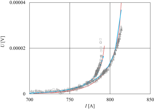
Figure 17. Current–voltage curves measured on one of the tested samples in two different cooling conditions compared with the theoretical prediction (37) assuming the hot spot length 2 mm and its critical current of 685 A and n = 25 (dotted lines). The results of numerical iterative computation using the same parameters (full lines) exhibit good agreement as well. Squares plot the data registered in the standard cooling conditions, while triangles show the results obtained at enhanced cooling. One can see that the theory nicely predicts the observed impact of cooling.
Download figure:
Standard image High-resolution image
Figure 18. The same data as in figure 17 plotted in log-log scales. The dashed line represents the current–voltage curve of the superconductor at the coolant temperature T0 considered in computations.
Download figure:
Standard image High-resolution imageA reasonable coherence between the theory and the experiment, including the vertical shape of U(I) dependence [133] at Itr, was found for all the experiments presented in figure 13 when the measured samples were suspended in liquid nitrogen. Nevertheless, in some trials with enhanced cooling, when the ceramic plate touched the measured sample from the bottom, a behavior deviating from theoretical predictions was observed. As an example, the experimental data for the defect with the lowest critical current are plotted in figure 19, together with the theoretical results obtained in the same way as in the previous case. The predictions for the thermal runaway in standard conditions, as well as the whole shape of the current–voltage curve, are plausible when assuming the weak spot parameters Δxws = 1 mm, Icmin = 154 A and n= 25. On the other hand, the value of Itr determined in the experiment with the enhanced cooling conditions the predictions of both theoretical models is exceeded by sim 3 A. An obvious candidate for explaining this discrepancy—save an experimental error—is an increase in the cooling mechanism stronger than the one observed in other cases, when the ceramic plate is put in contact with the tested sample. We intend to study this phenomenon systematically in the future; here it simply serves more as an illustration of how the analytical model presented in this paper could help in the investigation of a hot spot appearance in HTS tapes.

Figure 19. Current–voltage curves measured at two different cooling conditions on the sample with the lowest Icmin, compared with the theoretical expression (37) assuming Δxws = 1 mm, Icmin = 154 A and n = 25 (dotted lines). The results of numerical iterative computation using the same parameters are shown by full lines. One can observe a good quality of the prediction for the measurement in the standard cooling conditions (squares), but there is some discrepancy in the prediction for the experiment with enhanced cooling (triangles).
Download figure:
Standard image High-resolution image
6. Conclusions
The local reduction of critical currents in some spots of an HTS conductor is a phenomenon with a significant impact on the design and operation of devices like high-field magnets or FCLs for the DC grid. In contrast to low-temperature superconducting wires, the spread of the normal zone is slow, and the conversion of a weak spot into a hot spot is local and rather quick. In this paper, we present a complete theory that allows us to predict the limits of a safe operation of an HTS conductor with a local weak spot. Besides the weak spot length and its critical current, the conductor architecture, in particular the amount of stabilizing metallic layers, and the conditions of cooling play an important role. It is obvious from formulas (14) and (25) that the value of local critical current influences neither the maximum stable temperature, Ttr, nor the maximum of local dissipation, Ptr, before entering into the thermal runaway. On the other hand, the weak spot dimension could have an impact: we have found that a very small weak spot will never convert to a hot spot because of the heat removal along the conductor length. In this regard, the main role of the stabilizing layers is in thermal conduction, which could be improved also by adding non-metallic layers.
The set of formulas, allowing to identify the conditions of the thermal runaway, is finalized with the prediction (32) of the maximum DC that the weak spot allows to tolerate. Surprisingly, for the typical architectures of CC tapes designed for the magnet coil and for the FCL applications, this prediction differs less than what we have expected. From figure 11, where the results of our theory are presented for two realistic cases of cooling in a liquid nitrogen bath, one can see that the thermal runaway could appear at the DC exceeding the critical current in the weak spot, Icmin, by roughly 10%–25%. The preliminary analysis which we have carried out indicates that this conclusion is rather robust and remains true for the HTS coils operating at low temperatures too. The most difficult task, however, would be a valid estimation of Icmin at the lack of reel-to-reel conductor characterization in the operating conditions.
The validity of theoretical expressions has been verified in experiments on a set of samples with weak spots characterized by a wide range of critical currents. In the search for a tool that allows us to analyze not only the instant when the thermal runaway starts but the whole process of quasistatic increase of temperature at the current transport, we have modified the result derived in [70], and obtained the working formula (37). It predicts the shape of the current–voltage curve in realistic experimental conditions i.e. with the temperature rise caused by the local dissipation. A detailed analysis of the experimental data revealed several important features. The impact of hypothesized values of weak spot parameters Δxws, Icmin and n can now be verified in a much wider range of currents. As a result, the sensitive fitting of theory to experimental data allows a rather convincing deduction of the possible weak spot properties, also in case of a missing Ic (x) information. Likewise, our formula allows a quantitative prediction of the change of slope in the measured current–voltage dependence because of the sample heating due to the DC transport. Rather disturbing is the finding that the power exponent derived through the processing of experimental data without the examination of a possible sample heating—which is probably a quite common case—could be wrong by the factor as large as 2. A detailed experimental work combining the current–voltage measurement with the determination of temperature in the locations with the lowest critical current would be very helpful for a better understanding of this phenomenon.
Acknowledgments
This work was supported by the European Union's Horizon 2020 research and innovative program under Grant No. 721019, by the grant agency VEGA under contract 1/0151/17, and by the Slovak Research and Development Agency under Contract No. APVV-16-0418.
: Appendix
Properties of materials at cryogenic temperatures have been collected in several comprehensive sources [134, 135]. However, particularly for metals, these depend strongly on the processing and on the microstructure. Therefore, presenting the actual values used in computations [136, 137] is necessary for a cross-check verification. For this purpose, we report which data were used in the computations presented in this paper in the table 2.