

Abstract
The overall 30 year Nb3Sn conductor program for ITER provides an unusual opportunity to look at the issues created by the application of novel Nb3Sn technology on a large scale. ITER design criteria have evolved to make use of the features of the industrialized material, exploiting advantages as well as managing the disadvantages. There are lessons from the successes and failures to be learned for the future application of very high current Nb3Sn strands in fusion and high energy physics. The behaviour of Nb3Sn strands in the large compound ITER conductors is still producing surprises after 25 years of development, industrial production and testing, with the Nb3Sn strain sensitivity and brittleness producing many more subtle design impacts than originally foreseen. The results now obtained at the end of the ITER production suggest that, as a novelty for Nb3Sn, there are options for conditioning the strands in the ITER conductors that can be applied during commissioning and which could reduce the impact of brittleness by as much as one third.
Export citation and abstract BibTeX RIS
1. Introduction
The ITER project, a next generation superconducting tokamak capable of producing thermonuclear fusion, is presently under construction in France, with first operation expected in 2025–6. It is an international collaboration which has contributed to a long design and manufacturing process, in addition to the technical complexity of the machine. ITER selected Nb3Sn strands for the Toroidal Field (TF) and Central Solenoid (CS) Coils in the first conceptual design phase 1988–1991, setting performance parameters in 1993 that acted as a driver for industrial development over the following 25 years. These performance parameters were a key driver of the overall tokamak parameters. Following qualification by model coil tests in 2001–2, conductor production for the TF and CS coils started in 2007 [1] and was completed in 2015 with an overall production of about 700t of strand material [2].
The behaviour of Nb3Sn strands in the large compound conductors (with about 1000 individual strands of diameter about 1 mm cabled together and contained in a jacket) used in ITER is still producing surprises after 25 years of development, industrial production and testing [3–5]. The problem can be traced to two issues
- (1)The extreme strain sensitivity of the critical current in Nb3Sn [6].
- (2)The brittleness of Nb3Sn material under tensile strain [7].
Because of the difficulty in knowing the real strand strain state, the first produces uncertainty in expectations of what should be the performance of the compound cable based on that of the individual strands making it up, even if the filaments are not mechanically damaged. This may or may not be termed 'degradation', which we will anyway here call Type 1 Degradation. The second is more obviously a degradation because it can be linked to physical damage, but is still uncertain because of the unknown (and very complex) strand strain state. We will call this Type 2 Degradation. Type 2 Degradation is invariably associated with Type 1 Degradation and can be difficult to separate from it. Type 1 degradation may occur without Type 2 and is an inherent feature of many (if not all) large Nb3Sn multi strand conductors.
Already since 2002 we had evidence of a 'degradation' issue with the Nb3Sn conductors, initially thought to be Type 1 but eventually in 2013 Type 2 was definitively identified as well from filament micro cracking in the strands due to mechanical loads [3, 8]. A number of recovery programmes were implemented and followed from 2003, with varying degrees of success, and with increasing constraints from the on-going industrial production. These recovery programmes were initially focused on limiting Type 1 Degradation but after 2010 a programme to control Type 2 degradation in the CS conductors had to be put in place.
The CS micro-cracking issue (i.e. Type 2 Degradation) was resolved by cable modifications in 2013 [2], although as can be seen later, there is evidence that Type 1 is still present. These cable modifications could not (because of the production status) be implemented on the TF conductors.
Investigations completed in 2018 and reported briefly in section 4 finally confirmed that the TF conductor, with micro-cracks (Type 2 degradation), has sufficient margins left after stabilization of the degradation to meet the ITER requirements. An ongoing set of tests based on conductor samples is aimed at improving operational management of the Nb3Sn micro-cracking in the TF coils. The results suggest that, as a novelty for Nb3Sn, there are options for conditioning the strands in the ITER conductors that can be applied during commissioning and which could reduce the impact of micro-cracking by as much as one third.
The overall 30 year Nb3Sn conductor program for ITER provides an unusual opportunity to look at the issues created by the application of novel Nb3Sn technology to a large scale application, balancing the provision of stable requirements to industrial partners with the need to adapt to technical problems, over a period of 25 years. ITER design criteria have evolved to make use of the features of the industrialized material, exploiting advantages as well as managing the disadvantages. There are lessons to be learned both in the future application of very high current Nb3Sn strands, where the mechanical limits of very large Nb3Sn filaments are likely to produce more surprises in application of the strands, and in the future development of HTS materials where the material ductility has similarities to Nb3Sn. Many of the difficulties we have had to overcome in the ITER Nb3Sn production have been created by a drive for high critical current, neglecting the engineering usability of the strands. Identifying and understanding the dominant cost drivers in advance would have allowed us to get much the same result but much more quickly and cheaply.
2. Background I: history of Nb3Sn in fusion
Magnetic confinement of a hot plasma is a keystone of any magnetic fusion device and the generation of a high magnetic field with resistive conductors requires a very significant energy consumption that makes the efficiency of such devices impractical. Superconductivity allows to generate high magnetic fields with much lower power input and therefore it was recognized as a critical factor to the success of Magnetic Fusion in the 1960s and since then has been actively adopted as a key enabling technology in the world of nuclear fusion.
The superconducting properties of the Nb3Sn compound were discovered in 1954 [9], 8 years earlier than the superconductivity of NbTi was observed in 1962 [10]. However, NbTi industrialization went much faster than Nb3Sn and NbTi became quickly the preferred material for superconducting magnets. This happened mainly because of its alloy nature that demonstrated ductile mechanical behaviour and, as a consequence, much easier manufacturability. On the contrary, the brittle structure of Nb3Sn intermetallic compound posed a significant challenge for both material cost and manufacturability of magnets. As a result the first superconducting fusion magnets, for example the Baseball II (LLNL, 1970) magnet mirror or T-7 (Kurchatov Institute, 1979), the first Tokamak with superconducting magnets, that were designed in the 60 s and then constructed and commissioned in the 70 s, utilized solely NbTi superconductors [11, 12].
The situation started to change later in the 1960s when it was revealed that Nb3Sn in fact exhibits superconductivity at higher magnetic fields and therefore is able to carry a larger current than NbTi as both upper critical field and critical temperature of Nb3Sn are significantly higher (see figure 1) [13]. Understanding of Nb3Sn potential sparked interest in the fusion community to use higher magnetic fields and serious attempts to manufacture Nb3Sn superconducting magnets started [14].
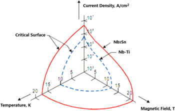
Figure 1. Critical surfaces of NbTi and Nb3Sn superconductors.
Download figure:
Standard image High-resolution imageSome of the first generation of superconducting fusion devices launched in 1970s like the mirror fusion test facility (MFTF) [15] or Tore Supra [16] were still relying on NbTi superconductors while attempts were being made to utilize the potential of Nb3Sn higher performances. As examples, a Nb3Sn Insert Coil was integrated in MFTF [15] and tokamaks T-15 and TRIAM-1 constructed in the Kurchatov Institute and the University of Kyushu correspondingly utilized mainly Nb3Sn superconductors [17, 18]. In addition, 5 large coils were constructed of Nb3Sn superconductor between 1979 and 2001 as technical demonstrators of material and design feasibility or as test facilities. These were: a D-shaped coil by Westinghouse for the large coil task collaboration, the demonstration poloidal coil Test Facility, SULTAN, Central Solenoid (CSMC) and Toroidal Field Model Coils (TFMC) [19–22]. SULTAN and CSMC have been functioning as test facilities for many years and have contributed invaluably to the knowledge of high field superconducting magnets that we have today.
Even though a significant experience of working with Nb3Sn had been gained during the projects mentioned above, Nb3Sn has not become a widely utilized material for fusion devices (see table 1). The most recent two generations of tokamaks (the 2nd, from the 1990s and the third, from the 2000s) culminating in JT60SA [23] launched during the 2000s in parallel with ITER construction, rely dominantly on NbTi. Of the 2nd and 3rd generations only ITER and KSTAR use dominantly Nb3Sn strands [24, 25].
Table 1. Nb3n consumption in tokamaks in the last 30 years.
| Facility | Year of commissioning | Weight of Nb3Sn t |
|---|---|---|
| T-15 | 1987 | 15 |
| KSTAR | 2008 | 23.5 |
| JT60SA | 2020 | 11.5 |
| ITER | 2025 | > 650 |
Use of NbTi clearly contributes a lot to cost saving as it is much cheaper than Nb3Sn but it cannot be the only reason for NbTi popularity in fusion since Nb3Sn offers potentially much higher plasma performance in a more compact machine. Due to its brittle nature Nb3Sn may demonstrate some performance degradation during operation and is prone to raise unexpected manufacturing issues. This feature of Nb3Sn had been recognized during the ITER Engineering Design Activity (EDA) 1993–2001 (see figure 3), however its quantification by detailed investigation was not deep enough as Nb3Sn use was not widespread and the data was not sufficient. ITER, with its enormous magnetic system and unprecedented consumption of Nb3Sn, has been the largest application of Nb3Sn ever. This massive use of Nb3Sn allowed an extended collection of valuable information in order to understand the material, its shortcomings and how to deal with them in future machines. Comparison of Nb3Sn consumption for major fusion facilities is shown in table 1.
3. Background II: development of Nb3Sn conductors for the ITER machine
The ITER conductor used in the superconducting coils of the Magnet System was ultimately chosen in 1993 as a rope-type cable-in-conduit conductor (CICC) made of Nb3Sn for the two high field systems (TF coils, CS coils) and of NbTi for the three lower field systems (Poloidal Field coil, Correction Coils (CC), Feeder busbars) cooled by a forced flow of supercritical helium. The cable is formed by multi-stage twisting of superconducting strands, with the final stage (except for the CC and busbar) consisting of 6 bundles twisted around a central cooling channel. The cable is enclosed in a stainless steel pipe or jacket that is formed from an assembly of butt-welded seamless pipes [2]. A cross-section of TF conductor and its opened out contents are shown in figure 2.
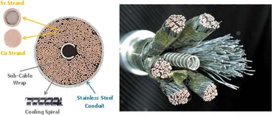
Figure 2. TF conductor cross-section (left) and exploded TF conductor (right).
Download figure:
Standard image High-resolution imageThe major design drivers for the ITER conductor design and the selection of Nb3Sn as superconducting material for TF and CS magnets were the high operating current of the magnet systems and correspondingly high magnetic field on the windings of magnets, to provide the magnetic flux to drive the plasma and a high field at the plasma axis. As ITER will produce several 100 MW of fusion power, nuclear heat dissipated on the TF inboard leg was a design consideration. A central cooling channel made of open stainless steel spiral provides improved cooling of the superconductor and the use of Nb3Sn provides (at least without Type 2 degradation) a large temperature rise capability. Both factors contribute to a heat extraction capability of several 10 s of kW from the TF coils, allowing ITER to compensate for inadequacies found in the nuclear shielding as designs matured to manufacturing reality.
Development of superconductors for ITER was started in 1988 in the framework of ITER Conceptual Design Activities (CDA) and 5 years later in 1993 the CICC concept was officially adopted. The years following 1993 involved different experiments with multiple superconducting coils to define final conductor layout as well as a level of required strand performances. In 2002 it was recognized that performances of Nb3Sn conductors selected for ITER may exhibit some irreversible degradation under cyclic electromagnetic loads [26, 27]. A margin to mitigate this degradation was included when requirements to strand and conductor performances were finally fixed in 2003.
However the base strand performance requirements of ITER were fixed in 1994 and did not change significantly up to the start of production in 2008. This period of 15 years allowed suppliers of Nb3Sn superconductors to focus on improving unit lengths and yield (avoidance of random breakage), both critical to minimize strand wastage in making large composite conductors, and, therefore, base the cost of the material on its weight and not on current carrying ability as has been usual for the high energy physics (accelerators) applications [28].
Over this period ITER required a Cu:nonCu current density of around 650 A mm−2 at 12 T and 4.2 K. This was near the top of suppliers capabilities in 1993. By 2008 Nb3Sn at 3000 A mm−2 could be produced, albeit not very cost effectively.
An overview of the main events of the ITER conductor development overlaid on the ITER project phases is shown in figure 3. The main events show in particular the consolidation of multiple conductor concepts to that shown in figure 2, in 1993 [29] and the discontinuation of the most exotic jacket materials (for example Incoloy 908 [30]) which had been selected with the objective of optimizing the strand strain in the conductors but in fact drastically complicated the coil manufacturing, in 2003. As will be seen in later sections, several major corrective actions still had to be implemented during manufacturing.
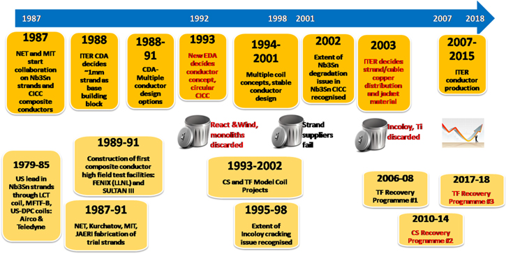
Figure 3. Timeline of ITER Project Nb3Sn Conductor Development. CDA: ITER Conceptual Design Activity, 1988–1991, EDA: ITER Engineering Design Activity, 1993–2001, Construction Phase 2007=>) FENIX and SULTAN III see [20, 29] NET: Next European Torus see [31].
Download figure:
Standard image High-resolution imageProcurement of conductors was started in 2007 with the first supply contract, or Procurement Arrangement in ITER terminology, signed. ITER need of conductor was provided through 11 Procurement Arrangements signed between ITER and 6 out of 7 international partners (China, Japan, EU, US, South Korea and Russia). 7 out of 11 Procurement Arrangements were dedicated to Nb3Sn based conductors: 6 for TF Conductors and 1 for CS Conductor, the remainder for NbTi. Supply of Nb3Sn conductors was perceived as a strategic technology for future fusion reactors and this overrode cost optimization considerations [2].
All requirements for conductor layout and manufacturing processes were strictly specified forming a build-to-print specification. Only the Nb3Sn strand process and internal layout were not specified and suppliers were invited to design and manufacture strands that would meet the defined requirements. Requirements for the superconducting Nb3Sn strands are provided in table 2. The final suitability of strands for ITER purpose was verified by testing a short conductor performance qualification sample in the Sultan facility [32] close to the coil operating conditions (except for strain).
Table 2. Requirements to Nb3Sn strands for ITER.
| Item | TF strand | CS strand |
|---|---|---|
| Minimum piece length | 1000 m | |
| Un-reacted, Cr-plated strand diameter | 0.820 ± 0.005 mm | 0.830 ± 0.005 mm |
| Twist pitch | 15a) ± 2 mm | |
| Twist direction | right hand twist | |
| Cr plating thickness | 2.0 + 0 −1 μm | |
| Un-reacted, Cr-plated strand Cu-to-non-Cu volume ratio | 1.0 ± 0.1 | |
| Residual resistivity ratio of Cr-plated strand (between 273 and 20 K) | >100 (after heat treatment) | |
| Minimum critical current at 4.22 K and 12 T | 190 A | 220 A |
| Resistive transition index at 4.22 K and 12 T | >20 in the 0.1-to-1 μV cm−1 range | |
| Maximum hysteresis loss per strand unit volume at 4.22 K over a ± 3 T cycle (for a sample greater than 100 mm) | 500 mJ cm−3 | |
In total there were 8 suppliers manufacturing Nb3Sn strands for TF conductors. 4 out of 8 suppliers selected the Bronze Route process while the other 4 opted for Internal Tin technology. The diversity of TF strands cross sections is presented in figure 4. Subsequently a 9th company, Furukawa, joined to manufacture a portion of Nb3Sn strands for the CS with other portions split between Hitachi and KAT [2]. The strand layouts have a common form, with an inner core containing the superconductor material enclosed by a diffusion barrier (Nb or Ta). The Nb3Sn strands produced industrially contain thousands of Nb filaments surrounded by a source of tin (pure or alloyed with copper). Outside the barrier there is high purity copper stabilizer with an outer Cr coating to control AC losses that would otherwise result from strand to strand contact in compound cables.
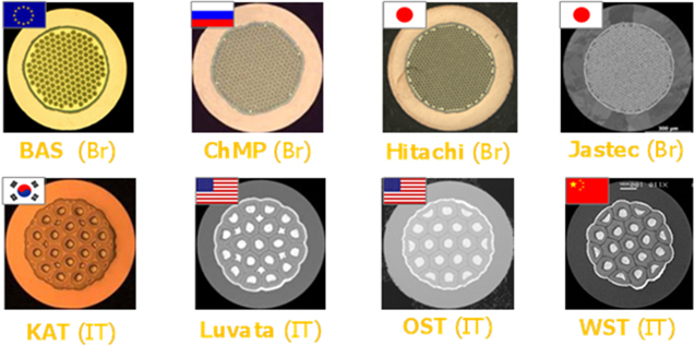
Figure 4. Cross-section of TF Nb3Sn strands (0.82 mm in diameter).
Download figure:
Standard image High-resolution imageA critical basic requirement was introduced by ITER in 1993 with Nb3Sn, that any strand could fit any conductor. This still holds and perhaps is the largest single contributory factor to the success of ITER strand production: engagement of many suppliers at an early stage. Down-selection of suppliers is often seen as an industrial strategy to reduce costs, overlooking that it creates losers and monopoly suppliers in the future. The ITER strategy of involving all who could qualify was much more successful, reducing the ultimate supplier risk and uncertainty and providing a good base for the future. In order to verify this assumption every combination of strand/cable/jacketing supplier underwent qualification—manufacturing of 100 meter long conductor with obligatory assessment of its performance in the Sultan facility [32] under near operational field and current conditions, through the test of a short (3.5 m) full size conductor sample.
The first strand contracts were signed early 2008, and production started early 2009 but took 2 years to ramp up achieving more than 100 tons per year in 2011. Production dashboards of TF and CS Nb3Sn strands are provided in figure 5. In total almost 700 tons of Nb3Sn were manufactured by the ITER partners for TF and CS Conductors.
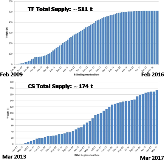
Figure 5. Timeline of Nb3Sn manufacturing for TF and CS strands.
Download figure:
Standard image High-resolution image4. Issues and recovery actions with the ITER Nb3Sn conductors
The mechanisms of Nb3Sn conductor Types 1 and 2 degradation in some of the ITER coils are discussed in the next section. In this section, we will consider the main coil tests which demonstrated the degradation (or its apparent absence) and the successive steps that were undertaken to try to eliminate Type 2. As will be seen, this elimination was only successful in the case of the CS conductor [33]. In addition to the main coil tests there were many conductor tests to try out modifications. These are not covered here except for the recent extensive set of TF conductor tests investigating management and mitigation of the irreversible degradation reported in sections 6 and 7. With the exception of the TFMC [23] these tests relied on the CSMC test facility [34] and its insert coils, as illustrated in figure 6. This facility provides a background field on a single layer insert coil of up to 13 T with conductor currents up to 70 kA in the insert coil.
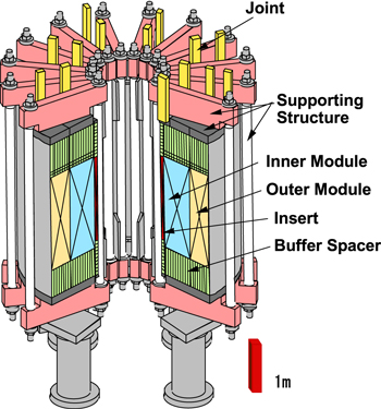
Figure 6. CSMC test facility, with insert coil.
Download figure:
Standard image High-resolution imageTable 3 shows the considerable variation in the 'conductor in coil' behaviour. It includes both Types 1 and 2 degradation but, as will be seen later, Type 2 degradation is associated with a higher performance loss and a much longer time (in terms of EM and WUCD cycles) before stabilization. Of the coils in the table, only CSI-1 and TFI-2 show clear Type 2 behaviour and only CSI-2 shows only Type 1 behaviour. To put in perspective the drop in current sharing temperature, the Nb3Sn coils in 2003 in ITER were designed with a 1 K temperature margin. The level of decrease particularly in the TFI-2 is then a major concern since, unless the conductors have some extra margins, the coils will be operating above the current sharing temperature.
Table 3. Summary of conductor in coil verifications of iter conductor performance.
| Coil | Loading | Degradationa | Special features | Jacket materiaJl |
|---|---|---|---|---|
| CSI 1 2001 | 10 000 EM and 5 Q | ∼0.4 K, then stable | 3 sc strands in triplet, 45 mm fstp | Incoloy 908 |
| CSMC ly 1 2001–2019 | ∼150 EM and ∼10 WUCD | ∼0.3 K, then stable | 3 sc strands in triplet, 45 mm fstp | Incoloy 908 |
| TFI 1 2002 | 1000 EM at 50% load, 4 Q | No measurable change | Poor instrumentation and steel mandrel, 3 sc strands in triplet | Ti |
| TFMC 2001 | 50 EM and ∼10 Q | n in cable ∼5–10, no measurable degradation | 2 sc strands in triplet, 45 mm fstp | SS |
| CSI 2 2013 | 16 000 EM, 3 Q and 3 WUCD | n in cable 5–10, no measurable degradation | 2 sc strands in triplet, 20 mm fstp | SS |
| TFI 2 2017–2018 | ∼1200 EM, 5 Q and 9 WUCD | ∼1.4 K, then ∼stable | 2 sc strands in triplet, 80 mm fstp | SS |
aIn this table degradation is defined as the change in Tcs from the first measurement on the coil (at full operational parameters) to the last. This ignores the probability that both Types 1 and 2 degradation occur on the first measurement cycle. WUCD: Warm Up Cool Down (300 or 80 K).EM: Electromagnetic Load Cycles.fstp: first stage twist pitch.Q: Quenches, typically to ∼100 K.SC: Superconductor.SS: Stainless Steel.
The test coils in table 3 did not have common cable configurations (nor common jacket materials, as listed in the table). Each coil test triggered modifications to the cable configurations, with the exception of the CSI-2 and TFI-2 tests which were tests of the as-built conductors. The main design changes are summarized in table 4 and illustrated in figure 3.
Table 4. ITER CS and TF cable design iterations.
| Date | Trigger | Changes | Result |
|---|---|---|---|
| 2003 | 2001 model coil tests showed degradation | Extra margin added for degradation, SS jacket selected to reduce risk of filament tension, Cu: non Cu fixed to 1.0 instead of >1.5 (cryogenic stability criterion abandoned), void fraction reduced | Large conductor cost reduction but degradation still found in 2006 conductor samples |
| 2007 | TF conductor tests showed EM degradation | Void fraction reduced, first stage twist pitch increased | EM degradation reduced |
| 2012 | CS Conductor tests in 2010 showed coupled EM and WUCD degradation | Coupled EM-WUCD degradation found, conductor trials show short twist pitch able to completely eliminate 'degradation'with EM and WUCD cycles | Implemented in CS but too late for TF |
We now know from destructive examination and quantification of filament fracture on Nb3Sn strands extracted from conductors that it is the local magnetic loads on a strands that cause the Type 2 degradation (compounded by axial thermal stresses) [7]. Taking as a very simple 'mechanical weight' (Field) × (StrandCurrent)x(first stage twist pitch), then table 5 shows (with hindsight) why the TFI2 and ITER TF conductor have the worst Type 2 degradation issues (i.e. it provides a simple post event explanation of the observations reported in table 4).
Table 5. Strand load characteristics in test coils (fstp: first stage twist pitch in m).
| Coil | B (T) | I(strand) A | BxIstxfstp |
|---|---|---|---|
| CSI 1 | 13 | 38 | 22 |
| CSMC layer 1 | 13 | 44 | 26 |
| TFI 1 | 13 | 39 | 23 |
| TFMC | 6.5 | 111 | 32 |
| CSI 2 (ITER) | 12 | 78 | 19 |
| TFI 2 (ITER) | 10.8 | 76 | 66 |
The final selection of the parameters for the TF conductor was made in 2008 based on analyses and the best conductor sample test results available at the time. The selected design relied on pseudo-long cable twist pitch (see figure 7). The Type 2 degradation issue of the ITER family (TF and CS) of conductors was eventually fully resolved in 2012/3 by the use of short twist pitches as in the CS conductors. However, the results of the crash programme carried out by IO for the CS conductors were not available when the TF conductor design was finalized and production launched (b).
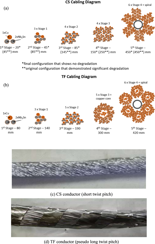
Figure 7. Cable diagrams of (a) CS and (b) TF conductors and examples of the different petals (c) and (d). The differences in the first stage twist pitch (top 45 mm, bottom 80 mm) are clearly visible.
Download figure:
Standard image High-resolution imageFigure 7 shows the as-built ITER CS and TF conductors. The strands used are similar, and in some cases identical, but the cables exhibit dramatically different performance, as shown in figures 8 and 9 which summarize the performance testing of the CSI-2 and TFI-2 coils.

Figure 8. Summary of main CSI-2 results: (a) Tcs, (b) extra strain, (c) n (all versus EM and WUCD cycles), also compared to the corresponding SULTAN sample (CSJA6). 'CSI Star' refers to a cluster of voltage taps on the CS insert used to derive the average electric field.
Download figure:
Standard image High-resolution image
Figure 9. Summary of main TFI-2 results: (a) Tcs, (b) extra strain, (c) n (all versus EM and WUCD cycles) also compared to the corresponding SULTAN sample. 'TFI Star' refers to a cluster of voltage taps on the TF insert used to derive the average electric field.
Download figure:
Standard image High-resolution imageThe CSI-2 results show typical Type 1 degradation, characterized by a low(ish) n, much lower than the strand, and a rapid stabilization after a very few EM load cycles (as seen in the n values). Any drop in Tcs compared to a 'perfect' coil is difficult to resolve since it is buried in the uncertainty of the strand strain. TFI-2 shows typical Type 2 degradation, n is lower than the CSI-2 and many EM/WUCD cycles are needed to achieve stabilization.
5. Filament bending and fracture in Nb3Sn and assessment of extent
5.1. The design challenge
Nb3Sn superconductor properties are highly dependent on the lattice distortion of the Nb3Sn. Nb3Sn is also well known as a brittle compound that easily fractures under tension [35]. After forming the cable from the strands it (and the conductor jacket) are then heat treated for a few hundred hours at about 650 °C to form the Nb3Sn compound [2]. This on its own produces many challenges for the jacket material and the coil insulation. At 650 °C, some components of the conductor are formed 'new'(the Nb3Sn), some are unaffected (Ta), or unaffected if separate from Sn (Nb), some undergo some stress relaxation (the steel jacket) and some are fully annealed (Cu and bronze).
In ITER, strands have to be separated to allow Helium at ∼5 K to provide cooling, and to limit AC losses. But the strands must be strongly supported for magnet/thermal loads. Achieving the correct balance is extremely difficult, and, due to cost pressures, there is a tendency to err on the 'overload' side. Figure 10 shows the situation, with the loads.

Figure 10. Magnetic and thermal loads on an ITER cable in conduit conductor.
Download figure:
Standard image High-resolution imageThis configuration is difficult to analyse mechanically, especially when cables become large with more than 1000 strands. Typical early simple attempts are shown in [3] and more recent in [36]. Broadly the strands are compressed by the thermal loads and due to the curvature, bend sideways. The (sideways) magnetic loads then add to this bending.
The causes of conductor degradation were discussed extensively between 2002 and 2012, along with ways to mitigate/control/eliminate. Early work [6] focused on bending and non-uniform strand properties which created inter filament current transfer (Type 1 Degradation). By 2013 clear evidence was obtained [3] that in some conductors filament fracture is playing a major role (i.e. Type 2 degradation).
However, even at this point, the mechanism by which both thermal and magnetic cycles could contribute to fracture was not clear. Subsequent tests (including the ITER conductor samples in 2018, described in the next section) show clearly that at least in the ITER TF conductors, it is a result of mechanical coupling between electromagnetic (or I × B) loads and thermal compression. Deformation and cracking under one causes repeated deformation and cracking from the other when conductor undergoes a load or thermal cycle. It is a form of coupled buckling [3] which is likely to be related both to the copper stabilizer on the outside of the strands and mechanical weakening as filaments fracture on the inside.
The nature of the cracks, and their distribution, are clearly identified in [8]. Figure 11 shows the result of micrographs made from strands extracted from a cable. These examinations also suggest that it is the local magnetic forces that cause the fracture, not (as was previously expected) the cumulative pressure build up inside the cable from one side to the other. However, there are also indications in more recent investigations that the cumulative pressure can create damage too [37].
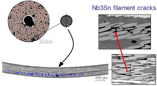
Figure 11. Visualization of cracked filaments (acknowledgement to Carlos Sanabria, Commonwealth Fusion Systems).
Download figure:
Standard image High-resolution imageUnfortunately, it is only possible to assess degradation with an I × B cycle, which makes separating the impact of thermal and magnetic cycles quite difficult. As shown in the next section, it appears that a thermal cycle is more critical than an electromagnetic one. Electromagnetic triggered degradation stabilizes after ∼10 cycles but is reset by each thermal cycle, which also stabilizes after ∼10–15 thermal cycles. This multiple dependency makes data reduction difficult, especially when trying to show visually a correlation between one of the measurements of degradation described below and the 'number of cycles'.
5.2. Assessment of the impact of bending and fracture
Since 2002, various methods have been developed to characterize the performance of degraded Nb3Sn strands [28]. The intent of all of them is to find a parameter that is independent of the strand operating conditions and can be deduced from the experimental data. The directly measured performance parameter is usually current sharing temperature but this is obviously dependent on current density and field, as well as being linked to the definition of the critical electric field at which it is measured. The two most useful measurements have been
- 1.Effective strain (sometimes as a function of electromagnetic load).
- 2.Fractured (or intact) filament area.
Both being supplemented by a deduction of the exponent of the resistive transition n which is defined below for a strand [14].
 where Ec (or E0) is conventionally 10 μV m−1
The total effective strain was originally developed [28, 30] because at least part of the strand degradation being observed (Type 1) was expected to be associated with current transfer. It is not reversible but nor is it fully what is expected as a 'degradation'. It is convenient because strand-in-conductor performance in Nb3Sn is always associated with a relatively unknown parameter, the filament strain. Lumping Type 1 degradation together with intrinsic strain and operational strain has the advantage of putting all the unknowns related to strain into one parameter. However, for Type 2 degradation caused by filament fracture, the effective strain is not a representative physical parameter, as it tends to vary with the operating conditions, and the fractured filament area appears more useful.
The second set of CS insert tests give a good example of a coil where using a strain based interpretation of performance, we find a dependence of extra strain on I × B, when operating strains are taken into consideration. The cable also shows, relative to the strand, a low n (although not as low as displayed in the second TF insert). The CSI-2 conductor showed low (negligible) filament fracture (as defined below) and no change with thermal or electromagnetic cycling. Therefore, there is no Type 2 degradation but significant pointers to Type 1.
The fractured filament area was first used in 2002 [26] and, because of its direct relation to the main factor behind the irreversible degradation found in the TF conductor, is the parameter used here. It is not entirely satisfactory since the filaments do not actually fracture to provide a full current transport barrier, but instead provide many (low) resistive interruptions to the current flow, where the nature of the current transfer depends again on the strand operating conditions. To derive the fractured filament area requires a knowledge of the Nb3Sn thermal and operational strain (εeff = εop + εth). Rather than (as above) deducing a total effective strain for the conductor based on the strand database and the coil measurements, the effective strain becomes an input parameter determined by a mechanical/thermal analysis. The deduced parameter is the fractured filament area. These strains are a form of average since the strains on the actual filaments are complicated by bending of the strands within the cable [3, 4, 6, 36].
Recent results from the ITER insert coils [38, 39] have finally reduced the uncertainty by confirming that the differential thermal strain between Nb3Sn and jacket (from 650 °C to 4 K) as well as the coil operational strains are 80% transmitted to the filaments [40]. The total strain in the TF conductor in operation at the peak field point is now assessed as −0.55% which includes any Type 1 degradation.
The fractured filament area is deduced from the coil performance measurements as follows
With jc(B, T, ε) coming from the strand parameterization (well defined for ITER, [2])

with L being the total length (direction z) over which the average electric field E(T) is being calculated, at a temperature T. Atot is the total conductor non-copper area, A is the intact non copper area and k is the fraction of the area that is intact. A and n are derived typically by measuring E(T) as a function of T and carrying out a best fit of the resulting curve, typically at E values from 5 to 50 μV m−1. Implicitly, n is not a function of B or T and is constant for all strands over the conductor. For single un-degraded strands (so n ≫ 10) n is well known to be a function of the critical current density but this dependence is expected to disappear in degraded strands.
Two items are critical to this process:
- 1.The availability of an accurate strand parameterization. During production of the ITER strands a very large effort was made to characterize the critical current of all types of strands, as a function of field, temperature and strain [41]. This work included cross-checking between laboratories carrying out the measurements and accurate parameterization of the results.
- 2.The knowledge of the cable strain state εeff. This is essentially including the Type 1 degradation before deducing the extra Type 2. This is obtained from pre-cycling measurements on the coils together with assessments from conductor samples of the transmission factor of operational and differential thermal strain to the strands [33].
The fracture filament area method was first applied to the first ITER CS insert coil [42] with the result shown below in figure 12. The order of fracture (25%–50%) is quite similar to that which will be estimated in later sections for the ITER TF conductors.

Figure 12. First ITER CS Insert Coil, 2001, fractured filament area estimates as a function of electromagnetic load cycles.
Download figure:
Standard image High-resolution image6. Degradation management I: extended tests on conductor samples
A number of questions come out of the coil tests, obviously directly relevant to ITER but also at a more general level. The ideal solution for ITER would have been (with hindsight) to make the TF conductor with a twist pitch of 20 mm, not 80. However, while this would have (probably) solved the ITER Type 2 degradation problem it leaves unanswered a number of more general questions, among them:
- (1)Does the CS conductor also reach a point (probably defined by electromagnetic load) where Type 2 degradation starts?
- (2)Is there any way now to 'manage' the TF conductor Type 2 degradation by (for example) limiting the operating current (or electromagnetic load) cycles as far as possible?
In the following sections we describe the investigations carried out at ITER with regard to question (2) and the results, which also have implications for (1).
6.1. ITER conductor samples
The ITER strand production was accompanied by a strong quality control programme that required the test of multiple full size Sultan conductor samples [2]. Since 2010 around one hundred have been tested. However, these samples were intended to be a form of production sampling, and were tested only at peak field and current, after a lifetime simulation of 1000 electromagnetic cycles (and one final thermal cycle that was not part of the acceptance test). This is in one sense an extreme form of EM loading since no part loads were carried out at the start, and in another sense optimistic, in that no intermediate Warm-Up, Cool-Down (WUCD) cycles were carried out. The risks in the procedure were indicated already in Sultan tests in 2012 but did not become fully known until the test of a second TF insert coil, TFI2, in 2017 [34].
This insert showed a pronounced degradation (certainly Type 2), with apparently a coupling between EM and WUCD cycles so that each WUCD cycle triggered a new set of EM degradations over the following 10 (or so) EM cycles before a stabilization. The loading was however again not representative of that to be imposed on the real coils, with a long series of full current full field EM cycles carried out before the start of WUCD, and only full current and full field EM cycles being performed. This insert eventually showed stabilization [39] but left open questions about the behaviour of different strands and the possibility of managing the Type 2 degradation as well as of course the mechanism causing the coupling between WUCD and EM cycles.
Since 2018 therefore, a series of new SULTAN samples have been tested with more realistic mixture of low EM cycles and WUCD than with model coils, insert coils and production conductor samples. These samples are made from the ITER conductor archive (2 samples are stored for every unit length). The aim was to look for thresholds for the onset of the WUCD-EM degradation cycles as well as to investigate the behaviour of strands from different suppliers. A summary table of these samples is given in a later section, table 6. In addition, some of the production samples [2] were similar to these recent samples and could be used for comparison. These appear in section 6.2 and are designated as TFEU8 and 10 and TFJA7 and 8.
Table 6. TFIO1 and TFIO2 results summary EM: Electromagnetic cycle, WUCD: Warm-Up, Cool-down cycle.
| Sultan sample | Strand type | WUCD (80 K) | WUCD (300 K) | 25% EM | 50% EM | 63% EM | 80% EM | 100% EM | Quench | Final Tcs, K |
|---|---|---|---|---|---|---|---|---|---|---|
| TFIO1R | Jastec | 14 | 14 | 140 | 120 | 120 | 120 | 120 | 8 | 5.6 |
| TFIO1L | Bruker | 14 | 14 | 140 | 120 | 120 | 120 | 120 | 8 | 5.7 |
| TFIO2R | Bruker | 2 | 10 | 80 | 40 | 40 | 40 | 80 | 3 | 5.9 |
| TFIO2L | Jastec | 2 | 10 | 80 | 40 | 40 | 40 | 80 | 3 | 5.6 |
| TFI-Sultan | Jastec | 0 | 2 | 0 | 0 | 0 | 0 | 1000 | 0 | 5.6 |
A typical example of the tests is shown in figure 13. Because of the coupling between EM and WUCD cycles, it is difficult to find a plot that enables trends to be picked out. In figure 13, both EM and WUCD are counted as 'equal' cycles. This at least shows the procedure that was followed but does not allow the different weight of EM and WUCD cycles to be observed. The plot shows that degradation sets in between 0.25 and 0.5 of the full load (current) × (field) kAT, BxI. It is worth noting that WUCD cycles in Sultan are a lot more time consuming (and expensive) than EM cycles. Even an 80 K WUCD takes 1 day; a 300 K cycle takes 3.
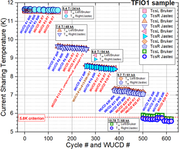
Figure 13. Sultan sample to investigate degradation, showing sequence of part load EM cycles and Warm-Up, Cool-Down (WUCD), together with the Tcs behaviour.
Download figure:
Standard image High-resolution imageOne of the overall features shown by these latest samples is that the degradation in current sharing temperature is either less than, or comparable to, the degradation found in the production samples. However, the production samples are subject to only one WUCD cycle and are clearly not stabilized. This opens the intriguing possibility that it is possible to condition (i.e. train) the Nb3Sn CICC conductors to better resist the combined magnetic and thermal load cycles.
6.2. Evidence of training
Evidence of training in Nb3Sn conductors is still subject to interpretation and further tests are needed to confirm it. Here we can set out, using the ITER TF conductor database, some of the evidence.
- (1)Thermal cycling of internal tin conductor during ITER production [43]
This was an early investigation of WUCD effects which was carried out in 2 steps. The sample has 2 identical legs, made of WST internal tin strand. In the first step, one leg (left) was subject to 10 thermal cycles to 80 K at the start and then to a further 30 cycles to 80 K before step 2 [43]. In the first step, both legs went through 1000 full current/field magnetic load cycles, in the second step both legs went through 3 × 300 K WUCD interspersed with 500 full current/field magnetic cycles.
Figure 14 shows the results. There is a difference of about 0.2 K between the two legs which is maintained over the life, with the 'thermally conditioned' leg remaining above the other leg. However, other samples from the same type of strand showed also a difference between the 2 legs that was maintained over the EM cycling and 1 WUCD [44]. So it is not clear if it is the thermal conditioning that is improving the Left Leg in figure 14, or a difference in the sample preparation. The difference in figure 14 is maintained through 2 WUCD whereas production samples generally converge with load cycling [45].
- (2)ITER conductor samples: trend comparisons
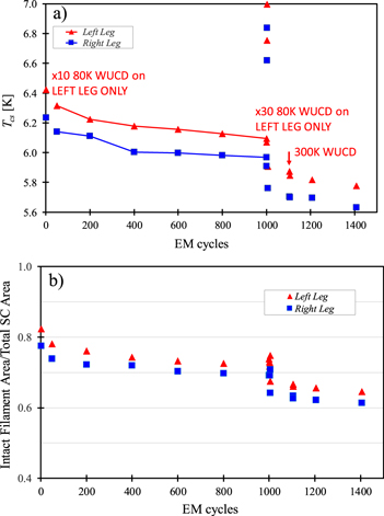
Figure 14. Test of an internal tin TF conductor with different thermal conditioning of the two legs. (a) Tcs measurements, (b) intact filament area assessment.
Download figure:
Standard image High-resolution imageAlthough several ITER TF conductor samples have been used in the degradation management programme, the training investigations have focused on two (both bronze route) where the samples have undergone testing up to full I × B and where there is a collection of production sample data available for comparison.
The TFIO1 sample was composed of two conductors based on bronze route strand. One of those was made by Jastec (JADA), the same strand used for the TFI manufacturing. The second leg was selected from Bruker-made strand (EUDA) that demonstrated the most similar performance to Jastec during qualification and production tests.
The sample was subjected to different combinations of thermal cycles (WUCD to 80 and 300 K) and electro-magnetic (EM) cycles as illustrated in figure 13. These increased the magnetic load progressively in steps from of 25%, 50%, 63%, 80% and 100% of the maximum EM load required in ITER.
The main goal of the TFIO2 test was to confirm the reproducibility of the TFIO1 results. Only 300 K WUCD cycles were implemented on TFIO2 during testing at lower EM combinations and then the effect of 80 versus 300 K was compared at the end of the campaign at 100% of EM load.
The final results are summarized in table 6. This table also includes the results of a 'TFI' sample which matched the conductor used in the second TF insert coil.
Table 6 shows clearly that TFIO1R and TFIO2L, although subjected to many more WUCD cycles, degrade to the same extent (or less) than the TFI sample.
TFIO1 and TFIO2 underwent, correspondingly, 28 and 12 WUCD cycles and that these WUCD cycles were mixed with different EM load levels. The TFIO1 and 2 are at or near stabilization after this. Production and qualification Jastec samples (81JNCxxx) were exposed to one WUCD cycle only and did not reach a stable level. There is a steep drop at the WUCD after 1000 EM cycles already close to the final level of the TFIO1 and 2, and this first drop may not have stabilized. The TFI samples were warmed up and cooled down a second time and already after this their Tcs is below that of the TFIO1 and 2 samples. This shows that the degradation of the conductor seems to decrease when the conductor is exposed to lower EM loads at the beginning of the testing series before being exposed to the highest ELM loads (i.e. a training effect).
The problem with quantitative interpretation of the test data is that there is an element of variability with single EM load tests and single WUCD, linked to delayed onset of fracture. A series of tests is much more reliable than an individual test. So in this section we have tried to find a way to look at trends rather than try to correlate changes with a specific cycle. This has the further advantage that the fairly large errors associated with looking at changes in intact filament area (or Tcs) between specific cycles can be reduced by looking at an overall trend.
To assess the data we have to find a way of simplifying the variability in cycles. There are too many parameters to enable trends to be established. The solution proposed is to define compound cycles. This concept follows from the observation that WUCD cycles, when followed by an EM cycles (unavoidable, to allow the extent of fracture to be measured) is much more severe than one (or 100) full load EM cycles. One conversion (of course, there are many possibilities) that gives consistent results is given below:
- One WUCD from 4 to 300 K and back to 4 K, followed by a full load electromagnetic cycle is defined as 1 compound cycle.
- 1000 EM cycles (whatever the electromagnetic load value) are defined as one compound cycle.
The contribution of a series of EM cycles is then determined by dividing their number by 1000. A WUCD plus the first EM cycle after the WUCD is weighted by (I × B)/(I × Bmax) with I being the conductor current and B the field, and additionally by 0.2 for an 80 K WUCD. This definition of compound cycles gives a reasonable similarity between TFIO1 and 2. Although there is no reason that the two should be identical, we could expect that they are at least similar in form.
A number of production samples are available for comparison with TFIO1 and 2, denoted as TFEU 8 and 10, and TFJA7 and 8. The definition of compound cycles normally reduces the production samples to 2 or 3 points (which was of course the reason for its definition, to take account of the higher degradation weighting found with WUCD than with EM). However, this limits the extent of the comparisons that can be made. To provide a wider set of data, an old production sample from 2012 (TFEU8) was reassembled in 2019 and put through further electromagnetic and thermal cycling.
Figures 15 and 16 show the results. The extended test of the TFEU8 production sample confirms the expected trend.
We can make some observations:
- On the first EM cycle after first cooldown, full load produces a drop of 0.3 of intact area (1 to 0.7–0.6), 0.25 full load produces a drop of 0.1 (1 to 0.9–0.8)-approximately.
- This difference is maintained throughout rest of life regardless of level of EM load (i.e. loading in steps reduces fracture by about 0.15).
- (3)ITER conductor samples: performance loss/cycle comparison
In order quantify better this (possible) training effect with a different assessment of the data, a performance loss indicator was defined and calculated for each series (at constant electromagnetic load) of TFIO1 and TFOI2 measurements. In line with the definition of 'compound cycles' above, the presentation focuses on thermal cycles followed by a few EM cycles, not on a long sequence of EM cycles. The initial Tcs value of a series was considered as T0, the final Tcs of the same series Tf. The difference between T0 and Tf is then divided by T0 providing the performance loss (%) = (T0 − Tf)/T0. For the TFI sample, the performance loss was determined for warm-up cool-downs only. To focus on compound cycles, Tcs at 1000 EM was taken as T0. The correlation of the performance loss with EM load cycles is presented in figure 17.
The results above confirm that the performance loss increases with EM load level, and that the conductors that were exposed to lower ELM loads first show a lower performance loss at the full (100%) EM load. The performance loss of the TFIO1 at 100% EM load is significantly lower than the TFI-Sultan sample, although the TFIO1 sample was subjected to 29 WUCD cycles, while TFI Sultan sample went through 2 WUCD cycles only.

Figure 15. EU Bruker strand, intact filament area versus compound cycles. Compound cycle = FAC * (I × B)/(68 × 10.78) or EM*0.001 where FAC = 1 for 300 K WUCD, 0.2 for 80 K WUCD, EM is any load cycle.
Download figure:
Standard image High-resolution image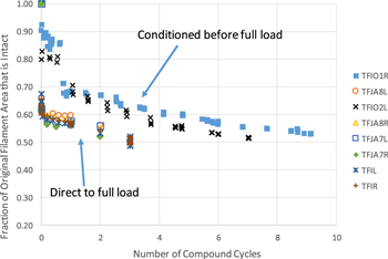
Figure 16. Jastec strand, intact filament area versus compound cycles. Compound cycle = FAC * (I × B)/(68 × 10.78) or EM*0.001 where FAC = 1 for 300 K WUCD, 0.2 for 80 K WUCD, EM is any load cycle.
Download figure:
Standard image High-resolution image
Figure 17. Sultan sample TFIO1, TFIO2 and TFI performance loss after different cyclic loads for a range of EM load (I × B) levels.
Download figure:
Standard image High-resolution image6.3. Possible mechanism for training
Although the test data indicates a possible training effect, that could be used to reduce the extent of filament fracture in coil applications, we also need to establish at least conceptually a possible mechanism for the effect.
The mechanism proposed is based around the mechanical behaviour of the copper outside the diffusion barrier that makes up about 50% of the area of the strand. Being furthest from the bending axis, the copper has also the largest potential impact on the bending stiffness of the strands.
The mechanical properties of Nb3Sn strands are dominated by the reaction heat treatment (at 650 °C) and the subsequent cooldown to 4 K [46, 47]. The copper in the strands is initially fully stress relieved and has a very low yield stress whereas the Nb3Sn (and any residual Nb material) are fully elastic even at 650 °C. As discussed in section 5.1, the copper is fully bonded to the unyielding Nb3Sn/Nb/Ta components which contract much less than the steel, and do not yield. In the cable, the strands can undergo bending (see figure 10) due both to the thermal loads (longitudinal) and the magnetic loads (transverse) [46]. This bending creates tensile strains, even though the Nb3Sn is compressed by the steel jacket. The Nb3Sn deforms elastically under this bending up to the point when it fractures, a tensile strain of around 0 to 0.002. The copper within the strands has a thermal contraction close to that of the steel jacket but, being attached to the Nb3Sn, is put into tension by it and due to its very low yield stress, it plastically deforms. The stress strain behaviour of copper at different temperatures is shown in figure 18 based on the mechanical property parameterization as a function of temperature given in [46]. Overlaid on these lines is the approximate stress–strain trajectory of the copper in the strands during the first cooldown. To produce this, we have assumed that the accumulated copper strain is one half of the integrated differential contraction from 650 °C, using the parameterization of the copper, Nb3Sn and steel thermal contraction reported in [46]. The copper work hardens substantially at 4 K and has a significant role in supporting the Nb3Sn filaments. So tensile strain on the copper may also be associated with filament fracture (of course, depending on the cable configuration).

Figure 18. Initial cooldown of cable, showing stress–strain trajectory on copper superimposed on copper elasto-plastic contours at constant temperature.
Download figure:
Standard image High-resolution imageFollowing this initial cooldown, it is possible to condition the conductor by carrying out thermal cycles from 4 K to either 77 or 293 K and then back to 4 K, or for the conductor to be subjected to EM loads immediately.
Figure 19 shows the approximate trajectory followed by the copper with this thermal cycling to 77 K. The situation is quite similar to a high temperature annealing process. Due to the bending, softening of the copper allows a strand deflection (in the form of a higher tensile strain). With 2–3 thermal cycles, the copper will stabilize on the 77 K stress–strain line.
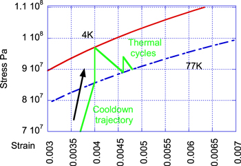
Figure 19. Impact of 2 thermal cycles to 77 K. Ratchetting and work hardening.
Download figure:
Standard image High-resolution imageFigures 20 and 21 show then the effect of an EM cycles with or without the thermal conditioning. We have assumed that the EM loads create an additional bending stress of 15 MPa. The copper that has been conditioned (i.e. work hardened) initially deforms elastically (due to the scale, this appears as a near vertical line) and then plastically. The un-hardened copper deforms immediately plastically, with the result that the copper at the end has a strain change under the EM loading of 0.0027, compared to 0.0005 with the work hardened copper. This translates into reduced Nb3Sn fracture for the conditioned strand.
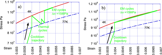
Figure 20. (a) Electromagnetic cycle after thermal conditioning, (b) electromagnetic cycle without thermal conditioning.
Download figure:
Standard image High-resolution image
Figure 21. Transition behaviour (I/Ic versus E/Ec) of superconducting strands. Typically Ec (or E0) is 10 μV m−1.
Download figure:
Standard image High-resolution image
These diagrams are of course largely qualitative and a gross approximation to the real mechanical situation in the strands, which is a mix of bending and direct stresses. However, they have a sufficiently quantified base to give confidence that a potential mechanism to explain the experimental results exists.
7. Degradation management II: revision of design criteria
7.1. Original criteria
The original design criteria for the ITER conductors were common to NbTi and Nb3Sn and were developed in the period 1988–1991 [44, 48]. They were based very much on the problems found in the 1980s largely with composite NbTi conductors and problems with stability [19]. The five factors considered were:
- (1)Cryogenic stability (Stekly criterion and limiting current) which gave Cu:nonCu requirements for the strands >1.5.
- (2)Quench and hot spot.
- (3)Derivation of Nb3Sn intrinsic strain based on differential thermal expansion with the jacket material from the heat treatment temperature, about 650 °C.
- (4)React and wind versus wind and react: maximum allowable strain on reacted strands.
- (5)Conventional temperature margin between operating temperature and current sharing temperature (defined by an electric field of 10 μV m−1) of >1 K for Nb3Sn, with a strand in cable n-value >20.
Nb3Sn conductors were being designed as if a kind of high field version of NbTi, leading to a failure to exploit the capabilities of Nb3Sn.
7.2. Limitations of criteria
These criteria were unsatisfactory in a number of respects, even with the extent of our knowledge in 1991. What we did not know then (or could not quantify, and therefore ignored) can be summarized as follows:
- The concept of Nb3Sn filament fracture except as an abrupt limit (below, no impact, above, fully broken and no current flow).
- Low 'n' behaviour (i.e. degraded) of Nb3Sn conductors and its impact on definition of critical current and operational regime.
- Current non-uniformity (inherent to any superconductor) and its effects on stability during pulsed (or even near steady state). There were several noted failures in the 1980s and the conditions to allow (or to block) current transfer between strands within a composite cable using strand coatings was the subject of much discussion in the 1990s with insulated strands still being proposed [49]. Eventually a Cr coating was selected for Nb3Sn and this has become standardized, allowing controlled and reproducible current transfer between strands in composite cables.
- The strain behaviour of the filaments inside the jacket. We expected significant gains in strand jc by choosing jacket materials that would allow the Nb3Sn to operate near the peak of the well known jc-strain curves [41]. Theoretically, based on differential contraction coefficients, the filaments in a steel jacket would experience a strain of −0.83% which reduces the jc from the peak of the curve by a factor of about 3 [35] whereas for a Titanium jacket the value is around −0.25% (and the jc is within 20% of the maximum value). Even in the 1990s, we expected some reduction of the 0.83% for steel, due to the impact of cabling, the positive effect of operation tensile strain and the extension of the jacket by the cable, hence the choice (rather arbitrary) of −0.5%.
The points at which these shortcomings were realized can be picked out in the timeline in figure 3 (the trash cans).
7.3. Formalization of new design guidelines
It was not until 2003 that we were able to obtain an agreement with (at that time) the only 3 ITER participants EU, US and JA to revise the Nb3Sn criteria to reflect the results of R&D in the 1990s and in particular the results from the ITER model coils 2000–2002 [21, 22]. The new guidelines were documented internally for ITER but have not been published as they have not been adequately generalized (i.e. they are applicable to variations around a specific ITER CICC). They can be divided into 3 groups with the last, the 'conductor-in-coil' reflecting the need for a more holistic approach to the conductor design.
7.3.1. Strand
- (1)The strand Cu:non Cu ratio was dropped from 1.5 to 1. Originally the strand Cu:nonCu ratio was fixed at 1.5 and above by the limiting current concept [50]. However, this is clearly not representative of the stabilization of low n Nb3Sn and so an alternative design rule is needed to select the copper fraction. This is now determined by the hot spot protection during quench and copper is provided where possible in the form of external strands (which are far cheaper than processing it along with the superconductor material in a superconducting strand). The value of Cu:nonCu ratio of 1.0 used for ITER was the lowest that the strand suppliers were comfortable to supply, while keeping RRR > 100. The copper plays an important role as a lubricant during strand drawing, and thin layers become easily contaminated during the heat treatment.
7.3.2. Cable
- (1)The base component of the composite cable, a triplet of strands, was changed from 3 superconducting strand triplet in TF and CS conductors to 1 Cu and 2 s/c strands.
- (2)The void fraction was reduced from about 36% to about 34%. This was an attempt to improve the support of the strands in the cable under the magnetic loads, and reduce the tendency to 'buckle' under the thermal loads. There is no direct experimental evidence that either of these objectives were achieved but the reduction in void fraction did not show any discernible negative consequences and produces a more compact conductor.
- (3)Allowed for low n-value in cable in the range 2–5.
- (4)The use of a short twist pitch for the first stage of the cable (composed of a triplet of the strands).
7.3.3. Conductor-in-coil
- (1)The TF conductor temperature margin was reduced from 2 to 0.7 K in 2003. Further simulations and operation of the test coils after 2015 have led to the practical abandonment of this criterion since stable operation can be achieved readily in low n Nb3Sn conductors even with a significant negative temperature margin. The conductor can be operated at any electric field as long as the cooling capacity is sufficient to extract the resistive heating without a thermal runaway developing. For the ITER TF conductors, with short high field regions, local electric fields up to at least 30 μV m−1 can be accepted.
- (2)Low carbon stainless steel jacket (to resist embrittlement in the heat treatment of the Nb3Sn) was chosen as baseline for the TF coils, and exotic material options such as Incoloy 908 and Titanium were dropped. The selection of strain conditions for the strands was based on test data from coil operation and not on expectations from differential thermal contraction coefficients.
These criteria reflect a move away from both cryogenically stabilized conductors and the historical treatment of a composite cable as a set of isolated strands. The separation of the copper from the strand in the first triplet is particularly important as a cost saving mechanism. The 33% saving in strand cost made a large contribution to cost reduction of >100 Meuro for ITER (at the strand prices at the time of around 600 €/kg). One of the penalties was the increase in magnetic loads on the strands by 50% which (for the TF conductor but not the CS) probably contributes to the degradation.
The situation with regard to temperature margin and stability is illustrated in figure 21. The superconducting transition does not represent a transition to current flow in the copper: this typically occurs at (E/Ec) > 10. At E = 10 μV m−1, the current flow is still very largely in the Nb3Sn and in the resistive matrix surrounding the filaments. At very low n the stability of the strand is determined by the stability of the heat extraction to the overall cable, not dynamic heat transfer from strand to local helium. Stable operation (with helium cooling) is possible up to at least E/Ec = 3 in ITER coils the TFI-2 was operated at 35 μV m−1 for > 30 min with a much lower Helium flow than in the ITER coils. Both Types 1 and 2 degradations (as long as controlled and stabilizing) remove the limiting stability issue and allow controlled exploitation of the resistive regime, inaccessible in NbTi.
8. Conclusions and lessons learned for the future of brittle superconductors
Overall, the production of high current conductor for ITER, covering the strand production, the cabling and the final integration of the strands into a conductor usable in a large coil, has been an outstanding success. The route to arrive at the point where completed coils are arriving at the ITER site has however been quite long and tortuous, essentially starting in 1988, and with several blind alleys. Even in 2019, during coil delivery, we are discovering new problems and new solutions to overcome them.
The overwhelming lesson from the 30 years of Nb3Sn development for ITER is that the issue is not the strand production but the strand use. An early lack of understanding of how Nb3Sn would work in a conductor and the critical differences to NbTi led to miss-focus on operating strand critical current as the driver of conductor 'acceptability' (and so dominating magnet cost), missing the critical manufacturability and integrated conductor performance issues.
With ITER, the drive to high critical current jc diverted attention for almost 10 years onto developing special conductor jacket material to optimize the Nb3Sn strain condition to give a high jc, creating numerous new problems which hindered the magnet design. The dominating issue of the sensitivity of Nb3Sn to strain and ultimately to filament fracture received little attention until almost too late for ITER and is still not fully understood. It will be interesting to see if the recent very high jc Nb3Sn strands can be successfully applied for HEP, since strain sensitivity is still present and an even greater sensitivity to fracture can be expected. The HEP magnets are less adapted to use 'slightly resistive' strands than the ITER ones.
Nb3Sn performance is dominated by controlling (or avoiding) filament fracture. It was avoided in the ITER CS conductor but will be very difficult to avoid with higher jc and higher field, with the pressure for more compact magnets with higher current strands, pushing the limits which therefore need to be understood. As long as filament fracture stabilizes, fracture need not be an issue and it brings opportunities to extend conductor operation far into a 'slightly resistive' regime that would be unthinkable with NbTi. Nb3Sn strand-in-conductor stability is different to NbTi and design criteria have yet to be derived. This paper contains suggestions on possible formulations.
Even when fracture is avoided, it appears that compound Nb3Sn cables inherently operate at low 'n' due to the strain sensitivity of the strand critical current. This occurs most easily within the strands but in cables with low contact resistance between strands, resistive current transfer between strands is also possible. The impact of this on the current density of the cable can be mitigated by recognizing the positive advantage it brings to superconductor stability, and designing for it at the start.
There are hints (quantified in this paper) that operational training (probably through the mechanism of work hardening of initially annealed copper) can improve filament support and reduce fracture for ITER. Such methods may bring benefits for extension of the operating regions of other magnets (or recovery when unforeseen problems are found). The investigation of the fundamental behaviour of Nb3Sn fracture mechanics (and current transfer) would repay investigation especially in high jc strands, much more than continuing pressure for higher current density in the 'non copper' area. It may be extendable to HTS material too. The mechanical design of strands-in-cables has been neglected and is critical to use of high jc strands at high field.
Acknowledgments
This paper is based on the work of many people in the ITER Organisation and the ITER Domestic Agencies who overcame many difficulties to successfully produce—and test—the conductors. Particular mention to Pierluigi Bruzzone and the SULTAN team, Lorenzo Cavallucci of the University of Bologna and Denis Bessette of IO, and the model coil and insert teams at QST Naka.
Disclaimer
The views and opinions expressed herein do not necessarily reflect those of the ITER Organization.