

Abstract
High-temperature superconducting (HTS) coated conductors (CCs) are frequently applied under complex electromagnetic fields to develop powerful, compact and efficient rotating electric machines. In such electric machines, field windings constructed by HTS CCs are adopted to increase the magnetic loading of the machines. The HTS field windings work with DC currents and due to the time-varying magnetic field environment, dynamic losses occur. In addition to the AC magnetic field, there is a large DC background field, which is caused by the self-field of the HTS field windings. This paper investigates the dynamic loss in HTS CCs using an H-formulation based numerical model for a wide range of combined DC and AC magnetic fields under various load conditions, and two different methods have been used for calculating dynamic loss. The results show that a DC background field plays a vital role to accurately predict the dynamic losses in HTS CCs. A DC background field of 75 mT can triple the dynamic loss as compared to only applying an AC magnetic field. In addition, the theoretical definition for the dynamic region for the case of solely an AC field has been found inapplicable in the case of a DC background field. Finally, a case study is done based on our double claw pole power generator to estimate the dynamic loss in an actual rotating machine, which was found to be 13.3 W. A low dynamic loss was achieved through the generator field winding design, which prevents high magnetic field fluctuations in the winding, since it is located at a distance from the air gap and armature coils. Furthermore, the rotational speed is very low and hence the resultant magnetic field frequency is low as well.
Export citation and abstract BibTeX RIS

Original content from this work may be used under the terms of the Creative Commons Attribution 4.0 licence. Any further distribution of this work must maintain attribution to the author(s) and the title of the work, journal citation and DOI.
1. Introduction
High-temperature superconducting (HTS) coated conductors are widely being researched in power applications. Especially for superconducting rotating machines, HTS CCs have become a promising candidate as opposed to conventional conductors to significantly increase the power densities [1–6]. HTS CCs are most commonly applied to the field windings of the rotating machine since they exhibit virtually no loss while carrying a DC current. However, due to the electromagnetic environment within the machine, dynamic losses occur [7, 8]. In this paper, a 2D multi-layer model, based on the H-formulation [9] is used to model the dynamic losses. While dynamic resistance and hence dynamic loss have widely been studied, most studies are done with solely an AC applied magnetic field [10–16]. However, when HTS CCs are applied to the field winding of superconducting rotating machines, there is a large DC background field, due to the self-field of the superconducting field coils, which affects the superconducting tapes in the windings [17–19]. To get a more accurate representation of the dynamic loss in superconducting field windings, further research is required. In this paper, dynamic loss is investigated and quantified for DC, AC and combined magnetic field environments. Two methods are used to calculate the dynamic loss. The first method is based on the theoretical definition of the dynamic region, which is dependent on the load factor to quantify the loss [10]. The second method uses the average electric field over the superconducting tape cross-section to determine the dynamic loss [11]. Both methods have been compared with each other and with experimental results for a frequency of 26.62 Hz [10].
2. Numerical mode
To model the superconductor behavior, the E − J power law is used for the HTS layer [20, 21]:
where E0 is the critical electric field, defined as 10–4 V m−1, n is the power index and Jc (B) is the field dependence of the critical current density, which follows equation (2). Since perpendicular fields cause the majority of the loss [13] and only perpendicular fields are applied in this paper, the parallel field component and anisotropic field dependency can be ignored

where Jc0 is the critical current density in self-field, B⊥ is the perpendicular component of the self-field and the applied magnetic field with respect to the surface of the HTS tape and B0 is the characteristic field of the superconductor.
To evaluate the losses in the model, the commonly used H-formulation [22–24] is used, which comprises of the following equations, Faraday's law combined with constitutive law (3) and Ampere's law (6)

with

where Hs is the self-magnetic field of the transport current and Hext is the external field. The applied external field is a combination of AC and DC components as highlighted in equation (5)


The transport current is defined as

where S is the cross-sectional area of the CC and i(t) is a ramp function to ramp up the DC transport current to the required load ratio.
In this paper, two different methods are used to calculate the dynamic loss. The first method considers the dynamic region [10]. For a coated conductor carrying a DC transport current It under an AC magnetic field B, the transport current occupies the superconducting layer with width 2ia in the center, leaving the rest of the width (1 − i)2a free on both sides, where a is defined as half the width of the HTS tape and i is the load factor. This region is defined as the dynamic region, of which the concept is illustrated in figure 1.
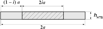
Figure 1. Dynamic region definition.
Download figure:
Standard image High-resolution imageHence, the average dynamic loss in the dynamic region per unit time can be calculated as

where T is the period of the applied magnetic field and Sdyn is the dynamic region as defined in figure 1.
The second method calculates the dynamic loss within coated conductors by using the average electric field as stated in [11]. The average electric field across the cross-section of the HTS tape can be defined as

and hence the instantaneous loss can be calculated with

where It is the DC transport current. The average dynamic loss per unit time (W m−1) can be given as

The two methods are used together to calculate the dynamic loss and are compared to experimental results. Details on the experimental setup may be found in [10, 14]. The tape parameters used in the model are shown in table 1. All the simulations were performed in COMSOL.
Table 1. SuperPower YBCO-coated conductor.
| Parameter | Variable | Value |
|---|---|---|
| Critical current | Jc0 | 2.63  1010 A m−2 1010 A m−2 |
| n-value | n | 22.5 |
| Magnetic field constant | B0 | 0.135 T |
| Tape width | 2a | 4 mm |
| YBCO layer thickness | hHTS | 1 μm |
| Substrate thickness | hSubs | 50 μm |
| Silver thickness | hAg | 2 μm |
| Total copper thickness | hCu | 40 μm |
3. Results and analysis
3.1. Perpendicular AC magnetic field
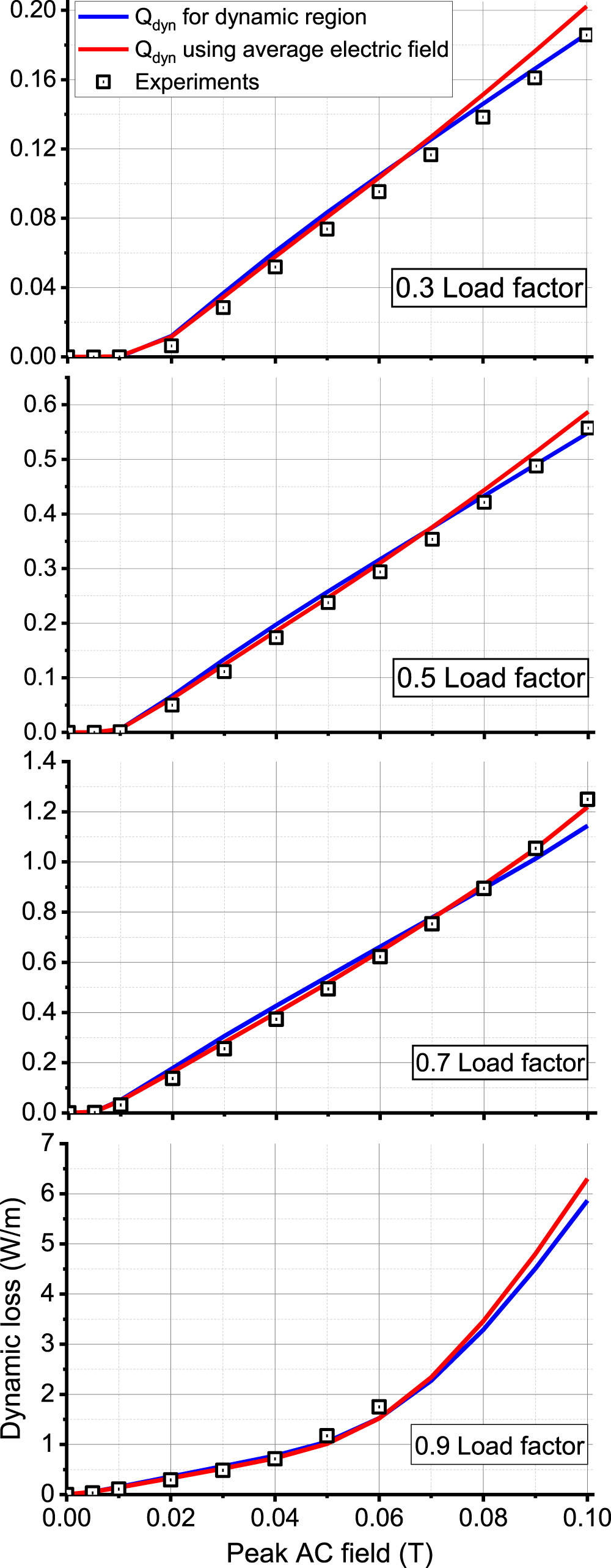
In this section, the dynamic loss results for applying a perpendicular AC field to the tape are shown in figure 2 for both methods and validated with experimental results. The frequency is set to 26.62 Hz and the respective load ratios are 0.3, 0.5, 0.7 and 0.9. The peak applied magnetic field ranges from 0 mT to 100 mT in 10 mT steps. As can be seen there is a very good correlation between the two methods and the experimental results. The dynamic loss is in positive correlation with the applied field as well as with the load factor.

Figure 2. Dynamic loss results for a load factor of 0.3, 0.5, 0.7 and 0.9 for the dynamic region and average electric field methods with experimental results. The applied field ranges from 0 to 100 mT in 10 mT increments. The frequency is 26.62 Hz.
Download figure:
Standard image High-resolution imageThere is no loss when the applied field is below the threshold field, after the applied field is greater than the threshold field, dynamic loss occurs and increases linearly with the applied field. There is a slight lift-off for a load factor of 0.7 and applied fields beyond 80 mT and a rapid increase in dynamic loss at a load factor of 0.9 for applied AC fields beyond 40 mT. The nonlinear behavior arises due to the field dependence of the critical current, which leads to Ic(B) dropping below the transport current IDC for short periods of time for each cycle leading to flux-flow loss [10, 14].
3.2. Perpendicular AC magnetic field with DC background field
Superconducting field windings in rotating electrical machines have a large DC background field due to the self-field of the field winding coils. To achieve a more accurate representation of the dynamic loss in superconducting tapes for applications such as in superconducting machines, a DC and AC combined magnetic field is applied to the HTS tape. As in the previous section, the investigated load ratios are 0.3, 0.5, 0.7 and 0.9. The applied AC magnetic field ranges from 0 to 100 mT in 10 mT steps with DC background fields from 0 to 100 mT in 25 mT steps. The results are shown in figure 3. It can be seen that for a low load factor, the DC background field only has a minor effect on the dynamic loss, since the transport current is relatively low, hence the reduced critical current, due to the field dependence, does not strongly affect the overall losses. As the load ratio increases, the dynamic loss increases significantly with the DC background field, due to the decreased critical current. While for the previous case, where no DC background field was applied, the nonlinear region for the dynamic loss only occurred for very high load factors and applied fields. When applying a DC background field of 50 mT, the nonlinear region already occurs for a load factor of 70%. Furthermore, in the previous case the rapid increase in dynamic loss only occurred for short periods of time each cycle when the AC field was in the vicinity of its peak, reducing the critical current temporarily below the transport current. Applying a DC background in conjunction with an AC field leads to the critical current being below the transport current for longer periods of time during each cycle, leading to a quicker and more rapid increase in dynamic loss. This becomes especially clear when comparing the loss results for the two cases where only a 100 mT AC field is applied and the case when only a 100 mT DC field is applied, both cases for a load ratio of 0.9. The dynamic loss result for the DC field case is significantly higher since the transport current is above the critical current for the whole cycle instead of only short periods of time as is the case for the 100 mT AC field example. While the two methods for calculating the dynamic loss show a similar trend, the method of defining the dynamic region as a function of the load factor leads to consistently lower results. This is due to the DC background field reducing the critical current, and hence, increasing the area that the DC transport current occupies. For a high load ratio of 90%, this effect is slightly mitigated since most of the cross-sectional area of the coated conductor is considered for calculating the dynamic loss. In addition, since the DC field direction does not change i.e. top to bottom, flux weakening and flux strengthening occurs on the edges of the tape, skewing the current and field distributions in the coated conductor. This is highlighted in figure 4, which shows the current density and magnetic field profiles for a 50% load factor, with an AC applied field of 20 mT, with and without a DC background field of 50 mT. For no applied DC field, the current density and magnetic field profiles are symmetrical and the dynamic region can be clearly defined as a function of the load ratio. With the applied DC background field, flux strengthening occurs on the right-hand side of the tape and flux weakening on the left-hand side, skewing the profiles towards the left. Hence, for more complex applied magnetic fields, it becomes more challenging to define the dynamic loss region accurately. Calculating the dynamic loss through the average electric field avoids this issue and leads to more accurate results.

Figure 3. Dynamic loss results for a load factor of 0.3, 0.5, 0.7 and 0.9 for the dynamic region and average electric field method. The applied AC field ranges from 0 to 100 mT in 10 mT increments with a DC background of 25, 50, 75 and 100 mT. The frequency of the applied AC field is 26.62 Hz.
Download figure:
Standard image High-resolution image
Figure 4. B and J profiles for a load factor of 50% and 20 mT applied AC field for (a) without DC background and (b) with a DC background field of 50 mT. The shadowed area is defined as the dynamic region.
Download figure:
Standard image High-resolution imageThe simulation results show that a DC background field such as present in superconducting rotating machine environments can play a vital role in the calculation of dynamic losses in superconducting tapes since it pushes the conductor into the nonlinear loss region for longer periods of time each cycle, leading to significantly higher losses. This is especially important to consider when operating with load factors beyond 70%.
4. Case study
To estimate the dynamic loss within a superconducting rotating machine, the double claw pole generator concept is taken as an example.
The double claw pole generator is a promising candidate to enable very large direct-drive wind turbines rated for 10 MW and higher due to its increased power density and hence lighter weight [25]. It features a stationary superconducting field winding, which is supplied with a DC current. Details on the cooling system of the HTS field winding can be found in [2, 26]. The design uses significantly less superconducting tape than other 10 MW superconducting generator designs [25, 26]. Rotating claw poles are oriented around the field winding to create a North-South pole flux variation along the stator coils on each side. The double claw pole generator concept is highlighted in figure 5. The main design parameters are highlighted in table 2. To further study the proposed design, the dynamic losses within the field winding need to be considered. For this purpose, a 3D transient finite element analysis was done using the simulation software MagNet to find the applied magnetic fields that occur on the surfaces of the field winding while the claw poles are rotating. The 2D HTS model introduced in this paper is then used to apply the resultant magnetic fields to the superconducting tapes, and hence determine the dynamic loss. This method allows to estimate the dynamic loss for the field winding without the need to build a complex 3D model of the whole generator, which includes the HTS properties, since the actual resultant magnetic fields in the generator are taken and applied to the superconducting tapes. This methodology also avoids the issue of the large aspect ratio of the field winding diameter (5.5 m) to the HTS layer thickness. Due to the very large size of the coil the 2D model is expected to be a good approximation to a full 3D model. To estimate the total dynamic loss for the field winding, the loss of each tape is then taken and multiplied by the required length depending on the location of the tape in the coil. Figure 6 shows a schematic of the field winding and the main points that were investigated are highlighted. As can be seen, the field winding consists of 3 coils that are placed next to each other. Splitting the field winding into several coils enables the generator to continue operating under partial load even if one field winding coil is damaged. In table 3 the superconducting tape parameters are summarized.
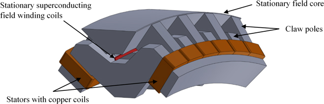
Figure 5. Double claw pole generator concept.
Download figure:
Standard image High-resolution imageTable 2. Double claw pole generator design.
| Attribute | Components | Value |
|---|---|---|
| MMF | HTS field winding | 32 400 A·turns |
| Active mass | 74 tonnes | |
| Mass | Structural mass | 115 tonnes |
| Total generator mass | 189 tonnes | |
| Dimensions | Outer diameter | 6.14 m |
| Axial length | 1.72 m | |
| Power output | 11.7 MW | |
| Performance | Rotational speed | 10 rpm |
| Power density | 61.90 W kg−1 |
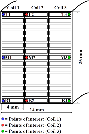
Figure 6. Cross-section of the superconducting field coil with highlighted points of interested.
Download figure:
Standard image High-resolution imageTable 3. Fujikura FYSC-SCH04 tape parameters.
| Temperature | 77 K |
| IC (self-field) | 230 A |
| n-value | 23 |
| B0 | 0.2 T |
| Tape width | 4 mm |
| Superconducting layer thickness | 1.9 μm |
| Substrate thickness | 75 μm |
| Silver thickness | 2 μm |
| Copper thickness | 40 μm |
The perpendicular flux density variation over one period for the investigated locations is shown in figure 7.

Figure 7. Perpendicular flux density variation for the investigated points on the field winding for (a) coil 1 and (b) coil 2.
Download figure:
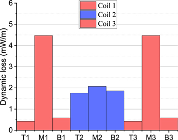
Standard image High-resolution imageThe generator design features 88 poles and rotates at 10 rpm, which results in an electrical frequency of 7.33 Hz. The peak flux densities occur on the edges of the coils, these values are taken and applied over the whole width of the relevant tapes to estimate the dynamic losses. Considering the reduced critical current due to the DC background field on the field winding, the transport current for the side coils (i.e. coil 1 and coil 3) is chosen as 52 and 122 A for the middle coil (coil 2), giving a load factor of approximately 0.7 for each coil. Figure 8 shows the dynamic loss results for the investigated coil locations.
Figure 8. Dynamic loss for investigated points in the field winding.
Download figure:
Standard image High-resolution image
It can be seen that the tapes in the middle of each coil have the highest loss due to seeing the highest magnetic fields. Since coil 3 sees the same magnetic field magnitude as coil 1, it is assumed that both coils exhibit the same dynamic loss. The loss for coil 2, i.e. the coil in the middle, is the lowest due to the shielding effect from the outer coils, it is affected by the lowest DC background field and only a small AC ripple. The total dynamic loss of the field winding may be estimated by multiplying the loss for each location by the required length of YBCO tape. The total current needed in the field winding is 32 400 A · turns, considering the transport currents, the middle coil is given 148 turns at 122 A, and the side coils 138 turns at 52 A. Hence, the side coils each require approximately 2.3 km of tape and the middle coil 2.5 km. The dynamic loss of the field winding can be roughly estimated to be 13.3 W, by multiplying the loss in each location of the coil by one third of the required length. Overall, the dynamic loss was found to be relatively low, since the rotational speed is low and hence frequency is very low. The dynamic loss increases along with the rotational speed. In addition, due to the design of the generator, the field winding coils only see small magnetic field variations, since they are located at a distance from the air gap and armature coils, which further reduces the dynamic loss. Under different load, this loss may change and should be considered for cooling system design.
5. Conclusions
Dynamic losses are particularly important for the design of field windings for superconducting rotating machines. In this paper the dynamic loss for YBCO CCs was calculated using two different methods for a combination of AC and DC applied fields. The first method calculated the loss over defining the dynamic loss region in function of the load factor. The second method quantifies the loss through calculating the average electric field across the conductor, which as a product with the transport current, gives the dynamic loss. The two methods have been validated with experimental results for various load factors and applied AC fields at a frequency of 26.62 Hz. It was shown that the DC background field significantly increases the dynamic loss due to the critical current dependency on the magnetic field. The average electric field method was found to be more suitable to quantify the dynamic loss since applying a DC field skews the current density and magnetic field profiles of the coated conductor. This complicates the definition of the dynamic region. Calculating the dynamic loss through the average electric field avoids this issue and leads to more accurate results. Finally, a case study on the double claw pole generator was done to estimate the dynamic loss for the superconducting field winding. The loss results were found to be relatively low, since the rotational speed is very low and due to the generator design, the field winding is only affected by small magnetic field variations. Overall the dynamic loss in the field winding was estimated to be 13.3 W.
Acknowledgments
This work was supported by the Engineering and Physical Sciences Research Council [Grant number: EPSRC EPN509644/1]. Hongye Zhang would like to thank the joint scholarship from the University of Edinburgh and China Scholarship Council under grant [2018] 3101.