

Abstract
High-temperature superconducting (HTS) flux pumps are promising devices to maintain steady current mode in HTS magnets or to energize rotor windings in motors and generators in a contactless way. Among different types of flux pumps, the dynamo-type flux pump has been very common due to its simple structure and ease of maintenance. However, understanding the principle of dynamo-type flux pump has been challenging despite the recent progress. This article employs an efficient numerical model based on minimum electromagnetic entropy production method to analyze the performance of the flux pump in open-circuit mode. This model is much faster and efficient than previous works on flux pumps. In addition to the main behavior of the flux pump, this work investigates the influence of airgap and critical current density on open-circuit DC voltage of the flux pump. We compare the modeling results of open-circuit DC voltage for different airgaps to experimental ones obtained in (Bumby et al 2016 Appl. Phys. Lett. 108 122601), showing good agreement. Modelling results show that with increasing airgap, pumping voltage in the superconducting tape does not cease, but only reaches to insignificantly low values, which is not measurable via experiments. In addition, the voltage in open-circuit does not depend on the critical current density, as long as the superconducting tape is fully saturated with screening currents.
Export citation and abstract BibTeX RIS
1. Introduction
Recent progress in the manufacturing technology of high-temperature superconducting (HTS) coated conductors (CC), paved the way for utilizing HTS CCs in magnets and power electric devices such as motors, generators and fault current limiters. The new generations of HTS conductors, HTS 2G conductors, are possible to be utilized under high critical current density (Jc) and magnetic field (B). However, applications with windings have been impeded in part because of thermal losses at the current leads and joule loss at joints. Although there has been some progress in the superconducting joint technology [1–3], there is still a long way to develop reliable and consistent superconducting joints with the similar HTS CC characteristics such as critical current, resistance and magnetic field dependence of critical current. In synchronous motors and generators, powering the pole coils at the rotor requires slip rings or brushes, adding additional problems to the aforementioned thermal loss. In addition, thick current leads in HTS motors and generators also imposes a considerable amount of heat and joule loss.
HTS flux pumps are devices that can be considered to address these problems [4]. They can be utilized to energize the HTS magnets to maintain the steady current mode or in rotor windings of electrical motors and generators to inject the current in a contactless way without using brushes. Another reason to avoid using brushes, which are a crucial part of off-shore wind turbines, is that they require continuous maintenance, which imposes extra costs.
Since 2011 when Hoffmann and et al proposed and designed the first traveling wave flux pump based on rotating magnets (dynamo-type HTS flux pump) [5–7], several articles have been published on performance, design and optimization of this type of flux pump. In [8], it was demonstrated that the function of HTS dynamo can be described by a simple circuit model including open-circuit voltage and internal resistance of the flux pump, which are closely proportional to its frequency. In addition, the flux gap between magnets and HTS tape is a critical factor. In [9], the performance of a simple HTS dynamo in open-circuit condition was examined and explained with a previously proposed model by Giaever [10]. The impact of stator wire width in an HTS dynamo type flux pump has been investigated in [11]. It is shown that the ratio of magnet width to stator wire width is a key factor for its design. Badcock and et al have shown that the efficiency of an HTS dynamo increases with a total magnet area and does not depend on the magnet orientation [12]. The Effect of frequency on output DC voltage of an HTS dynamo has been studied in [13]. It was found that there are three frequency regimes of behavior including low, mid and high regions. In [14], the effect of the number of rotor magnets and rotor speed on the performance of an HTS dynamo was examined. A linear relation was observed with the number of magnets and output open-circuit voltage and also short-circuit current. Hamilton and coworkers in 2019 studied the effect of synchronous and asynchronous number of magnets on the rotor of an HTS dynamo [15].
Due to the complexity of performance of traveling magnetic wave flux pump and in particular dynamo-type HTS flux pump, the details of its principle does not seem to be fully understood yet [16]. Moreover, an efficient, fast and yet precise modeling method can be a reasonable choice due to the following reasons: restrictions in experimental studies like measurement errors, difficulty in measuring some parameters such as magnetic field density and voltage, when the signal getting too weak to be measured, and most importantly the cost of designing and building apparatus along with conducting the studies. Besides, for better analyzing the complex principle of flux pump, studying the simpler cases such as open-circuit mode can be more suitable due to eliminating the effect of the current flowing in the HTS circuit.
There have been few papers that modeled the performance of HTS flux pumps. In 2017, a simple yet effective linear HTS flux pump was modeled with finite element calculations using a 2D A-formulation [17]. The model could successfully demonstrate the pumping performance of the flux pump although there were some drawbacks. First, the model did not regard a rotating magnet flux-pump but an artificial configuration of a moving C-shaped magnet. Second, that article used the critical state model with constant critical current density, Jc, to define the superconductor properties, and hence it lacked consideration of Jc(B) dependence, which is crucial in the process of flux pumping. In addition, using very limited time steps and also sudden vanishing of the magnet to generate pumping behavior made the model unrealistic and far from an experimental flux pump. In [18–20], the dynamic resistance in HTS coated conductors have been modeled using different methods in 2D. All these models were validated using experimental measurements. Since they have used stationary uniform sinusoidal ac magnetic field as external applied magnetic field, the case is completely different from the moving magnet, which creates a traveling non-uniform magnetic field. Therefore, dynamic magneto-resistance modeling cannot provide a realistic description of the mechanism of a dynamo-type flux pump. In [21], a transformer-rectifier HTS flux pump was modeled in COMSOL using a 2D H-formulation and verified by experimental data. However, that kind of flux pump is based on the dynamic magneto-resistance created by a stationary AC magnetic field, rather than traveling magnetic flux. Although the mechanism of generating voltage is similar to dynamo-type flux pump, there are significant differences between applying magnetic field in these two types of flux pumps. Then [21], is not representative for dynamo-type flux pumps. In 2019, Mataira and et al proposed the first model of a dynamo-type HTS flux pump using a 2D H-formulation finite element method in COMSOL [22]. They calculated the DC output voltage in open-circuit condition and showed that this DC voltage is due to the nonlinear eddy currents in over-critical condition, which forms the dynamic resistance. They also use realistic properties for the superconductor being and E − J power-law relation with Jc(B, θ) from transport measurements, where B is the magnetic field modulus and θ is its angle with the tape normal. Thanks to this, the modeled output voltages agreed with experiments. However, their model in [22], based on the H formulation, is very slow. This is because of the need to mesh the air and the complications associated to rotating mesh, necessary to model the circulating magnet. Indeed, the need of meshing the air in large regions is common in most finite element methods (FEM) [23].
In this article, we present a fast and accurate modeling method for a dynamo-type flux pump with realistic superconductor properties (E − J power-law relation with Jc(B, θ) from critical-current measurements on single tapes). For this purpose, we use the minimum electro-magnetic entropy production (MEMEP) method [24, 25]. This variational method solves the local current density as state variable, which avoids meshing the air and the associated difficulties to moving mesh. This fast and accurate model is very practical to analyze the influence of several parameters, which will ease the optimization of flux pump designs. Here, we focus on the effect of the air-gap and the value of the critical current density. For certain configurations, such as high airgaps, it is necessary to use many elements in the superconductor width, which was not possible for previous models due to high computing time [22]. To verify our modeling results we compare them with measurements for several air-gaps from [9], showing good agreement. This emphasizes the efficiency of the presented modeling method.
2. Modeling methodology
2.1. MEMEP 2d method
In this paper, the MEMEP method in two dimensions has been employed for modeling. This variational method is able to take materials with nonlinear E(J) relation like superconductors into account. MEMEP is based on the calculation of current density J by minimizing a functional containing all the variables of the problem, such as the magnetic vector potential A, current density J, and scalar potential φ. It has been proved that the minimum of this functional in the quasimagnetostatic limit is the unique solution of the Maxwell differential equations [25]. Since the current density is only inside the superconducting part, discretization of mesh in the domain around the superconducting region is not needed in this method. The general equation for the current density and the scalar potential are as follows:


The vector potential A in equation (1) has two contributions including Aa and AJ, which are the vector potential due to applied field and vector potential due to the current density in the superconductor, respectively. Here, 2D geometry has been assumed so that J = Jez and A = Aez. Furthermore, the Coulomb's gauge (∇ · A = 0) has been assumed, and hence for infinitely long problems AJ follows [23]:

For cross-sectional 2D problems with current constraints, equation (2) is always satisfied, and hence only equation (1) needs to be solved. To solve this equation, the following functional needs to be minimized [25, 26]:
where U is the dissipation factor defined as [25]

This dissipation factor can include any E − J relations in superconductors including the critical state model [25].
The functional is minimized in discrete time steps. If the functional variables are J0, AJ0 and Aa0 in a particular time step like t0, then on its next time step t = t0 + Δt, the variables will become J = J0 + ΔJ, AJ =  + ΔAJ and Aa = Aa0 + ΔAa, respectively, where ΔJ, ΔAJ and ΔAa are the change of the variables between two considered time steps and Δt is the time period between the two time steps. In this modeling, the non-uniform applied magnetic field Ba caused by the rotating magnet appears in the functional in the form of Aa [25].
As previously explained, meshing was performed only inside the superconductor region in rectangular shape elements and uniformly across the object. For this modeling, only one element along the thickness of the superconducting tape suffices and the optimum number of elements along the width was chosen to be around 200 elements for small gaps. This number has been increased up to more than 3000 elements, when higher precision is needed, especially in larger airgaps where the magnetic field density is weak. Therefore, the whole number of elements in the modeling was between 200 and 3200 elements, which reduces the computation time significantly compared to conventional FEM. Besides, the optimum number of time steps that were chosen were 360 per cycle, being the lowest number of time steps that the computations are independent on the number of time steps.. For this number of mesh and time step, the computation time was less than 20 min per cycle.
2.2. Magnet modeling
The vector potential and magnetic flux density generated by the magnet can be calculated by the magnetization sheet current density K = M × en, where M is the magnet magnetization and en is the unit normal vector to the surface. For uniform magnetization, the vector potential AM and magnetic flux density BM generated by the magnet are

where em is the unit vector in the direction of magnetization, ∂S represents the edges of the magnet cross-section, and dl' is the length differential on the edge. Note that since both em and en are in the xy plane, the cross-product em × en is always in the z direction, and hence A follows the z direction. In this article, the intergrals for AM and BM were evaluated numerically.
The magnetic field generated by the magnet acts as an applied field. Then, the program only needs to calculate this vector potential and magnetic field, once for each time step within the first cycle. The impact on the total computing time is negligible, since minimization takes most of the computing time.
2.3. HTS tape characteristics
To define the nonlinear superconductor characteristic, the model uses the isotropic E − J power law

where Ec = 10−4 V m−1 is the critical electric field , Jc is the critical current density and n is the power law exponent or n-value. With this E(J) relation, the nonlinear resistivity defined from E(J) = ρ(J)J is

For the E − J power law, the disspiation factor of the functional in the equation (5) becomes

The Jc(B) dependence of the critical current density of the HTS tape has been obtained from measurements in the temperature of 77.5 K (liquid nitrogen) performed in [22] and has been utilized in our model (figure 5). The tape critical current was measured in the range between 0° to 180° and the critical current dependence was assumed symmetrical from −180° to 0° .
2.4. Model geometry
The current density J flows in the z direction, and hence the vector potential A and electric field E are parallel to the z axis. The magnetic field B is perpendicular to the current density and its direction belongs to the xy-plane. Due to infinitely long symmetry, the following relations can be derived
Taking these relations into account and equation (1), it is found that

where ∂zφ is uniform within the superconductor. Since Coulomb's gauge is assumed, the scalar potential becomes the electrostatic potential. Figure 1, shows the sketch of the modeling configuration.
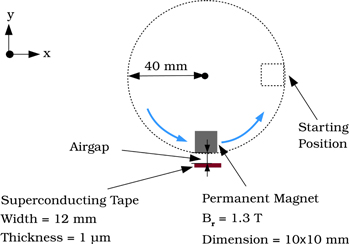
Figure 1. Configuration of the 2D model, where all components are assumed infinite in the z direction (perpendicular to the shown plane).
Download figure:
Standard image High-resolution image2.5. About the open-circuit voltage
To obtain open-circuit voltage, the gradient of the electrostatic potential needs to be calculated from equation (12).
In 2D modeling, the fact that the gradient of the electrostatic vector potential is uniform along the z axis, allows us to easily calculate the gradient per unit length. Afterwards, the voltage (or open-circuit voltage in our case) can be simply calculated by

where l is the length of the tape in between the voltage taps, which in the presented 2D modeling is related to the dimension of the used magnet.
3. General behaviour of open-circuit voltage
This section presents results of the open-circuit voltage calculation. The input parameters used for these calculations were obtained from [9] so that it can be comparable to the experimental results presented in the mentioned paper.
3.1. Parameter description
The permanent magnet used for this study is a square magnet with the dimension of 10 × 10 mm. Note that although in [9] a cylindrical shape of magnet has been used, the conversion of a cylindrical shape in 2D would be a rectangular shape, which of course is not a perfect transformation, but accurate enough for our estimations. Furthermore, as shown in [22], the flux pumping mechanism can be well explained by a 2D model. The magnet type is a N42 magnet (Nd–Fe–B magnet), which offers the remanence magnetic field of around 1.3 T.
The parameters that have been selected to model the YBCO superconducting tape are 12 mm width, 1 μm thickness, n-value 30, and critical current at self field as 281 A. The Jc(B, θ) data used for HTS tape were obtained from the experimental data in [22], which belongs to the same type of the HTS tape (not identical tape) as in [9].
The rotating radius of the magnet rotor is 40 mm and the magnet outer surface has been placed on the circumference of this rotor. The rotating frequency is 12.3 Hz. The set-up configuration has been shown in figure 1.
3.2. Main behavior
The results presented in this section were calculated for airgap of 3.3 mm. The airgap was defined as the distance between the magnet surface and the HTS tape. Using the procedure explained in section 2.5 the voltage was calculated considering the Jc(B, θ) dependence. Besides, all the results belong to the second cycle to skip the transient state in the first cycle. The calculations start with the zero-field cooling condition, being J = 0 at t = 0. We tested and verified that the results at the following cycles are the same as those at the second cycle.
The calculated output V is comprised of two terms

where A is the total magnetic vector potential and E is the electric field, which is obtained by the E − J relation considered for the HTS tape and is dependent on the local current density of the tape. For the modeled flux pump, this voltage V has been calculated in figure 2 during the second cycle.

Figure 2. Output open-circuit voltage in the airgap of 3.3 mm. The result belongs to the second cycle to skip the transient state.
Download figure:
Standard image High-resolution imageHowever, an important parameter for flux pumping is the dc voltage component, Vdc. This dc component is defined as follows
where l is the tape length and ρ is the nonlinear resistivity of HTS tape. In the equation above, the vector potential in steady state is used, which is periodic and hence ![${\int }_{0}^{1/f}{\partial }_{t}A\,=\,A[1/f]-A[0]=0$](https://content.cld.iop.org/journals/0953-2048/33/3/035008/revision2/sustab6958ieqn2.gif) . The cause of the periodicity of vector potential is that both A from the magnet and the currents in the superconducting tape are periodic after the first cycle.
. The cause of the periodicity of vector potential is that both A from the magnet and the currents in the superconducting tape are periodic after the first cycle.
Based on equation (15), the output Vdc only depends on the electric field generated by the resistivity of the HTS tape, which itself is a function of the tape current density. An interesting feature is that Vdc can be calculated from the time integral of ρ(J)J on any point, the integrals for all points yielding the same result. Then, we can also use the cross-section average of the electric field to calculate Vdc, being

where S is the cross-section surface and ds its differential. For the modeled flux pump, this contribution of voltage in the HTS tape is shown in figure 3.
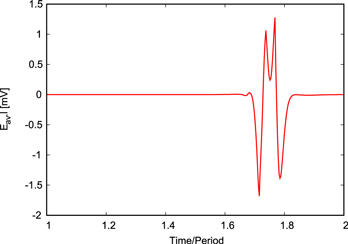
Figure 3. The generated open-circuit voltage by the nonlinear resistivity of the HTS tape in the airgap of 3.3 mm. Eav is the cross-section average of E(J) = ρ(J)J and l is the tape length. The result belongs to the second cycle to skip the transient state.
Download figure:
Standard image High-resolution imageThe instantaneous output voltage of a flux pump can be expressed as
where Aav is the average total vector potential in the tape and A = Aa + AJ where Aa is the vector potential due to external magnetic field and AJ is the vector potential due to local current density in the tape. Using the same arguments as equation (15), we find that the dc voltage follows

For a linear material we have

and hence Vdc vanishes for the open-circuit case because I = 0. However, Vdc does not vanish for the superconductor nonlinear E(J) relation.
The output voltage difference between the tape at 77 K (superconducting mode) and at 300 K (normal mode), being very relevant for measurments, is

which is equal to
For open-circuit mode, the last term vanishes. In addition, since the metal resistivities are large at 300 K, the vector potential generated by currents at 300 K (Aav,J,300 K) will be negligible compared to those from superconductor at 77 K (Aav,J,77 K). Therefore we will have

where the sub-index oc denotes the open-circuit mode.
If Vdc of the graph in figure 3 is calculated using equation (18), it can be observed that the flux pump has a DC value equal to 33.6 μV. Over many cycles, this value of DC voltage will be accumulated to inject the magnetic flux into a superconducting circuit connected in series to the pump [9]. In figure 4, this trend can be noticed over 10 cycles for the modeled flux pump. The accumulated voltage is calculated by


Figure 4. Accumulated open-circuit voltage over 10 cycles in the airgap of 3.3 mm.
Download figure:
Standard image High-resolution image3.3. Comparison of the cases with constant Jc and Jc(B, θ) dependence
The performance of the flux pump is also studied with the assumption of constant Jc at self-field. For this case, the generated Vdc in each cycle is equal to 16.2 μV, which is almost half of the case for Jc(B, θ) dependence. In this section, the reason behind this difference is investigated.
The flux pumping phenomena occurs because of overcritical eddy current generated in HTS tape while the magnet traverses over the tape [22]. According to the Ic(B, θ) data showed in figure 5, which was obtained from [22] and measured at 77.5 K in magnetic fields up to 7 T, the magnetic field significantly redueces the local Jc across the tape. For instance, in the case of airgap equal to 3.3 mm, the maximum perpendicular magnetic field density in the tape is around 260 mT (marked with blue dashed line in figure 5).
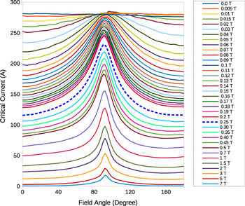
Figure 5. Experimental Ic(B, θ) data used in the modeling. Data was measured at 77.5 K in magnetic fields up to 7 T, derived from [22].
Download figure:
Standard image High-resolution imageFigure 6 depicts the comparison of the current density profiles, Jz, in the case of constant Jc (red solid line) and dependent Jc(B, θ) (blue dashed line) when the magnet is just on the top and middle of the tape with the airgap of 3.3 mm. Although the magnet is concentric with the tape, the current density is not symmetrical because of the hysteretic nature of the screening currents. In the case of constant Jc, the local Jc across the tape remains the same (green dashed line in figure 6). Therefore, the overcritical eddy currents that results in generation of electric field, and thus voltage, belong to the regions where the red solid line exceeds the green dashed line. However, in the case of considering Jc(B, θ) dependence, the value of Jc will diminish up to around 0.8 of Jc in the middle part (yellow dashed line in figure 6), due to perpendicular magnetic field density up to 260 mT. Therefore, the overcritical current occurs in regions where the blue dashed line exceeds the yellow dashed lines. Experiments and modeling results confirm that the latter leads to higher amount of electric field and voltage generated by the flux pump.
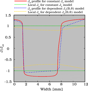
Figure 6. Comparison of the Jz profile from the constant Jc model (red solid line) and dependent Jc(B, θ) model (blue dashed line) when the magnet is just on top of the tape and concentric to it with airgap of 3.3 mm. Green and dash yellow lines show the local Jc for constant and Jc(B, θ) dependence, respectively.
Download figure:
Standard image High-resolution image3.4. Effect of tape critical current
In this section, we investigate the impact of the critical current density of the HTS tape on the generated open-circuit voltage of the flux pump. We consider several different cases with constant Jc with critical currents ranging from 70 to 1120 A, including the experimental critical current in self-field of 280 A. The rest of the parameters are the same as in the previous sections.
Figure 7 shows the signal of Eavl for three different values of Jc corresponding to critical currents of 140, 280 and 560 A. An important result is that this signal is almost the same, taking into account the high variation of Jc. The cause is that, as long as the tape is saturated with magnetization currents, only the value and time dependence of the magnetic field from the magnet is important. When looking at the DC component, which is responsible for flux pumping, the difference is even smaller (table 1), being almost no difference for Ic between 70 and 560 A. The decrease in the DC voltage at 1120 A is expected to be due to significant shielding of the magnetic field from the magnet, since the self-field is of the order of 100 mT and the maximum magnetic field from the magnet is around 250 mT (see figue 9).
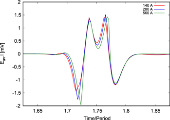
Figure 7. Comparison of the generated open-circuit voltage in the airgap of 3.3 mm for tapes with different Jc, corresponding to the Ic values in the legend. The signal is for the second cycle, in order to skip the transient.
Download figure:
Standard image High-resolution imageTable 1. Calculated DC voltage for different Jc values, assuming constant Jc in the tape.
| Ic (A) | DC voltage (μV) |
|---|---|
| 70 | 15.5 |
| 140 | 15.9 |
| 280 | 16.4 |
| 560 | 15.3 |
| 1120 | 11.1 |
4. Airgap dependence of open-circuit voltage
The DC component of the open-circuit voltage is the same as that of ΔV as defined in equation (20), since the normal-state contribution at room temperature vanishes. This is convenient because measurements can easily determine ΔV, which in open-circuit mode can also be calculated from equation (22). As it is illustrated and showed by experiments in [8, 9], ΔVoc decreases with increasing airgap, which is the result of reduction of magnetic field density in the tape. Figure 8 shows the calculated results demonstrating the reduction of ΔVoc for the modeled flux pump from 2.4 mm up to 50 mm. The shape of ΔVoc also qualitatively agrees with the experiments performed in [22] and, in particular, the increase of the second positive peaks compared to the first and the shift of the positive peaks to the right.
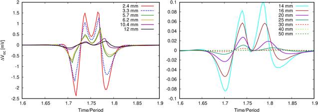
Figure 8. Calculated results showing the trend of reduction of ΔVoc with increasing airgap up to 50 mm (ΔVoc ≈ l[∂tAav,J + Eav]). The case with airgap of 3.3 is marked with blue dashed line (left plot).
Download figure:
Standard image High-resolution imageThe magnitude of magnetic field density plays an important role in creating voltage in the flux pump. Figure 9 depicts the trend of reduction of maximum perpendicular magnetic flux density in the tape with increasing airgap in the range of 0.5–50 mm. By increasing airgap, the maximum perpendicular magnetic flux density in the tape decreases sharply and, accordingly, the reduction of ΔVoc is predictable. Indeed, the magnetic field generated by the magnet at high distances is approximately the same as an infinitely-long dipole, which deacays as 1/r2 at high distances.

Figure 9. Magnitude and trend of reduction of the maximum perpendicular magnetic flux density in the tape with increasing airgap.
Download figure:
Standard image High-resolution imageWe may wonder what is the boundary for generating voltage in a flux pump. In other words, what is the maximum airgap that results in non-zero voltage in the flux pump. This issue is directly related to the value of magnetic flux density on the tape surface. Figure 10 demonstrates the change of open-circuit DC voltage generated in the modeled flux pump for airgaps up to 50 mm. That figure indicates that even in airgaps as large as 50 mm, DC voltage still exists; while the maximum applied perpendicular magnetic field density is of only 7 mT. Although this value is insignificant, i.e. around 0.0002 μV, it suggests that there is still voltage generated in the flux pump. Considering the fact that the maximum perpendicular magnetic field density of 7 mT is much less than the penetration field (Bp) estimated for the modeled HTS tape in the flux pump (i.e. 25 mT) [5], it can be concluded that the generation of voltage in flux pump does not require full penetration of the field into the tape, but only partial penetration can lead to voltage generation. For confirming this claim, figure 11 depicts the current density profile with airgap of 50 mm, when the magnet is just on top of the tape.

Figure 10. Although the DC open-circuit voltage in the flux pump decreases with the airgap, it never vanishes. Calculated voltage for the cases of constant Jc and magnetic-field dependent Jc(B, θ) for airgaps in the range of 2.4–50 mm.
Download figure:
Standard image High-resolution image
Figure 11. The current density line diagram when the magnet is just on the top of the tape with airgap of 50 mm. The encircled areas show the overcritical regions of current density.
Download figure:
Standard image High-resolution imageFigure 11 indicates that the full penetration of the magnetic field has not occurred in the tape when the magnet is on top and in the closest distance to the tape. However, there are some small regions where the current density profile exceeds the local critical current density in the tape. Note that in here, due to the very small perpendicular magnetic field in the tape, the local critical current density is almost the same as the critical current density at self-field Jc0 (yellow dashed line in figure 11). These regions can be responsible for generating the insignificant value of voltage observed in figure 10.
Figure 10 also shows that for constant Jc the DC voltage is almost the same as for Jc(B, θ) for gaps from 16 mm and above. This indicates that for this gap, the magnetic field from the magnet is much smaller than the self-field, suggesting that this kink is caused by the influence of the self-field. We also tested the sensitivity of the results with the number of elements (up to 3200 cells in the tape), the tolerance of J, the number of time steps per cycle, and the accuracy of the interaction matrix; finding that the results in figure 10 do not change after improving any of these numerical parameters.
4.1. Quantitative comparison to experiments
To confirm the modeling results, the DC value of the open-circuit voltage for different airgaps have been compared to experimental studies obtained from [9], which can be observed in figure 12.

Figure 12. Comparison of modeling results with experimental studies performed in [9] for the DC value of open-circuit voltage for different airgaps.
Download figure:
Standard image High-resolution image
From figure 12, it is apparent that there is good agreement between DC values for airgaps equal to or larger than 3.3 mm. However, there is a big discrepancy in airgap of 2.4 mm. The reason for this discrepancy can be explained by several factors. The first one, as explained before in section 3.1 comes from the shape of the magnet. The magnet used in experiments was cylindrical while in 2D it is not possible to model this shape and, instead, the square bar shape has been used. This difference becomes bolder when the magnet gets very close to the tape because the shape of flux lines in very close distances are different in cylindrical and infinite rectangular magnets (the modeled one). The other error originates from measurements. This mostly happens due to error in measuring airgaps because of thermal contraction and also changing airgap value during movement of the magnet. In the end, also the modeling error cannot be neglected. This partly originates from the limitations of 2D modeling and assuming infinite tape and magnet in z direction (modeling was performed in xy-plane), and hence the flux lines are not identical to the real magnet. The variations of Jc(B, θ) within the measured tape could also cause discrepancy.
5. Conclusions
Dynamo-type flux pumps, which belong to the category of traveling magnetic wave flux pumps have become popular due to its simplicity and ease of maintenance. In this work, a numerical method based on MEMEP has been utilized to model a dynamo-type flux pump. This model solves the Maxwell equations only inside the superconducting region with minimization of a functional. Thanks to this, it is efficient and fast, which provides the opportunity to model more complex geometries and parameter sweeps. The principle of flux pumps do not seem to be fully understood yet and studying open-circuit mode is more helpful to understand its mechanism, because it is simpler compared to full-circuit mode. By analyzing the DC open-circuit voltage in the airgap range between 2.4 and 50 mm, we found that the DC voltage generation does not cease even in large airgaps up to 50 mm, where the maximum perpendicular magnetic field density is around 7 mT. The reason can be justified from the existence of overcritical regions near the tape edges even under small values of magnetic field, which leads to the generation of DC voltage in the HTS tape. The comparison between modeling results with experimental studies obtained from [9] in the airgap range between 2.4 and 10.4 mm shows good agreement with experiments. We also found that the generated voltage in open-circuit for constant Jc does not depend on the Jc value, as long as the tape is fully saturated by screening currents and the magnetic field that they generate is much smaller than the magnet field. This modeling method can open the way for fast and reliable studies in order to further analyzing the behavior of flux pumps and for optimizing their structures.
Acknowledgements
We acknowledge C Bumby and R Badcock for discussions and for providing the previously published measurement data. This work received the financial support of the Grant Agency of the Ministry of Education of the Slovak Republic and the Slovak Academy of Sciences (VEGA) under contract No. 2/0097/18.