
Abstract
Stacks of superconducting (SC) tapes can trap much higher magnetic fields than conventional magnets. This makes them very promising for motors and generators. However, ripple magnetic fields in these machines present a cross-field component that demagnetizes the stacks. At present, there is no quantitative agreement between measurements and modeling of cross-field demagnetization, mainly due to the need for a 3D model that takes the end effects and real micron-thick SC layer into account. This article presents 3D modeling and measurements of cross-field demagnetization in stacks of up to 5 tapes and initial magnetization modeling of stacks of up to 15 tapes. 3D modeling of the cross-field demagnetization explicitly shows that the critical current density, Jc, in the direction perpendicular to the tape surface does not play a role in cross-field demagnetization. When taking the measured anisotropic magnetic field dependence of Jc into account, 3D calculations agree with measurements with less than a 4% deviation, while the error of 2D modeling is much higher. Then, our 3D numerical methods can realistically predict cross-field demagnetization. Due to the force-free configuration of part of the current density, J, in the stack, better agreement with experiments will probably require measuring the Jc anisotropy for the whole solid angle range, including J parallel to the magnetic field.
Export citation and abstract BibTeX RIS

Original content from this work may be used under the terms of the Creative Commons Attribution 3.0 licence. Any further distribution of this work must maintain attribution to the author(s) and the title of the work, journal citation and DOI.
1. Introduction
Stacks of superconducting (SC) ReBCO tapes after magnetization behave like permanent magnets but with a superior trapped field, setting the world record of 17.7 T [1] compared to the around 1.3 T maximum remnant magnetic field of conventional permanent magnets. Although SC bulks can also trap high magnetic fields (17.6 T [2]), stacks present additional advantages. First, their Hastelloy substrate enhances their mechanical properties. Also, the stack length is virtually unlimited with very uniform Jc, and the stack width could be as wide as 46 mm [3]. Larger continuous SC shapes result in larger trapped flux for the same maximum trapped field. Following the critical state model (CSM), a saturated bulk mosaic made of hexagonal or square tiles traps an average flux density of around 1/3 of its maximum, while the average flux density on an stack is around 1/2 of its maximum [4]. Then, a long stack traps 50% more flux than an array of bulks of the same width as the stack for each bulk. In addition, the stack enables interlaying sheets of other materials to enhance physical properties: metal layers enhance thermal properties and soft ferromagnetic layers enhance the trapped field and reduce cross-field demagnetization, at least for stacks as stand-alone objects and below the saturation for the magnetic material [5].
The high trapped flux in SC stacks can be exploited to enhance the magnetic flux density at the gap of motors and generators, when placing these materials in the rotor [6–8]. Other alternatives to achieve the same goal by means of superconductors is to use bulks [9–12] or pole coils in the rotor [13, 14]. Higher gap flux densities enable weight and size reduction for the same power and torque ratings. This feature can be further enhanced by adding an SC stator [15–17], resulting in a full SC motor. Thanks to this, SC machines present a high potential [18], especially for electric aircraft [6, 16, 17, 19–22], high power generators [14, 22, 23], and sea transport [11–13].
For the stack of tapes' technology, the ripple transverse fields that the stacks experience in the rotor cause demagnetization of the trapped field, being a major issue. The acceptable level of demagnetization depends on the application. For aircraft propulsion, the rated power should be kept during commercial flights of a few hours. One option could be that at take-off the stacks are over-magnetized to trapped fields above the requirements, in order to guarantee the rated level throughout the flight. Then, we can estimate that demagnetizations above 30% in a few hours are impractical.
There has been a big effort to fully understand the cross-field demagnetization, in order to reduce demagnetization effects and extend the time of the trapped field inside the stack, as follows.
Recent measurements of stacks showed the main behavior under cross and rotating magnetic fields [5, 24–26], the latter reporting measurements for up to 10 000 cycles. However, theoretical study by cross-sectional approximation (infinitely long 2D approach) showed qualitative agreement only [5, 25]. In addition, [25] compares an A-formulation with Brandt–Mikitik theory [27], showing good agreement. One reason for the quantitative disagreement with experiments is the unrealistically high thickness in the models of 10–20 μm compared to 1–2 μm in the experimental samples. Liang et al take the real thickness into account in their 2D modeling, showing again good qualitative agreement but still quantitative discrepancies [28]. As stated in [28], the remaining discrepancy is due to the end effects of the relatively short experimental samples (usually made of square tapes), requiring 3D modeling. 3D models have been only published for cylindrical bulks by Fagnard et al [29] or cubic bulks by Kapolka et al [30]. However, a full 3D model of the stack of tapes is missing, where good qualitative agreement with experiments is expected. In addition, 3D modeling can also enable studying the current density component parallel to the ripple field, in contrast to 2D modeling, which can describe the perpendicular component only.
The main reason for the missing 3D models is due to the low SC thickness of around 1 μm and the need to mesh several elements across the thickness, resulting in a high aspect ratio of the elements. Since the variation of current density across the thickness is essential for cross-field demagnetization, methods assuming the thin film approach cannot be applied. The inaccuracy associated to the elongated elements leads to numerical issues such as a high number of elements, instability, and the non-convergence of the modeling tools. These are the reasons why models often do not take the real thickness of the SC layer into account.
Our goal is to model stacks with the real thickness of the SC layer (1.5 μm) and compare the results to measurements, becoming the first 3D model of the cross-field demagnetization of stacks of tapes. Thus, following the methodology definitions in [31], we 'attack a well-known problem at the frontiers of knowledge'. For the studied configuration, our method, the minimum electro-magnetic entropy production method in 3D (MEMEP 3D), is more efficient than the finite element method (FEM) in  formulation, because, due to the thin film shape, FEM uses many elements in the air around the sample and even between thin films [32]. In addition, certain software packages like COMSOL present issues for 3D elements with the required high aspect ratio. The stack cross-field configuration also seems unsuitable for fast Fourier transformation (FFT). The bulk FFT approach [33] requires a cumbersome number of elements due to the need for uniform mesh and the low film thickness. The stack approach of FFT assumes thin films for the tapes [34], which cannot describe cross-field demagnetization. Therefore, we model the experimental geometry by the MEMEP 3D method. Another advantage of the MEMEP 3D method is that it is able to take macroscopic force-free effects into account [35], backed by the theory of Badia–Lopez [36].
In this article we focus on the cross-field demagnetization of: stacks of tapes up to 5 tapes with the MEMEP 3D method, the validation of our MEMEP 3D method by comparison of 2 tapes demagnetization with FEM, the trapped field in the stack up to 15 tapes, and the qualitative behavior of bulks and stacks with similar parameters.
2. Methodology of measurements
The study is focused on the cross-field demagnetization of a stack of tapes. The sample is prepared from 12 mm wide SuperOx tapes with the stated minimum Ic of 430 A at 77 K. The thickness of the tape is around 65 μm with a 1.5 μm thin SC layer. The tape has ∼2 μm silver stabilization on each side and around 60 μm Hastelloy. The stack of tapes is formed by 5 SuperOx tapes with 3 Kapton layers between each SC layer. The SC tape together with three Kapton insulators is 220 μm thick. The sensitive part of the Hall probe sensor is 1.5 mm above the top SC layer. The sensitivity of the probe is at least 10 mV/T.
Cross-field demagnetization consists on the following three main steps: magnetization by the field cooling (FC) method, relaxation time, and cross-field demagnetization. The detailed process is the following:
- The sample is placed into the electromagnet at room temperature.
- The electromagnet is ramped up to 1 T.
- The sample is cooled down in liquid nitrogen bath at 77 K.
- The electromagnet is ramped down with ramp rate 10 mT s−1.
- The sample is moved into the air-core solenoid.
- The sample is left for 300 s relaxation.
- The Arepoc Hall sensor LHP-MPc is placed 1.5 mm above the sample measured the trapped magnetic field Bt at the center.
- The solenoid magnet applied a sinusoidal transverse- (or cross) magnetic field of several amplitudes (50, 100, and 150 mT) and frequencies (1 and 10 Hz). The Hall probe measured the trapped field during the demagnetization.
The measurement set-up contains a G10-cryostat for sample holder, an iron-core Walker Scientific HV-4H electromagnet, and the separated air-core solenoid (figure 1).
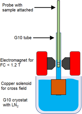
Figure 1. The measurement set-up magnetizes the SC stack by FC using an electromagnet and later applies alternating cross-field demagnetization by means of a copper coil.
Download figure:
Standard image High-resolution imageThe control system [26] contains a signal generator (Agilent 33220A) amplified by two power supplies (KEPCO BOP 2020) connected in parallel. The current in the circuit is measured by a LEM Ultrastab IT 405-S current transducer. The magnetic field is measured by an Arepoc Hall sensor LHP-MPc [37]. The circuit is monitored by custom made LabVIEW program.
3. Modeling method
In this article, we use two different numerical methods. Most of the calculations are made with the MEMEP 3D method, although we first benchmarked this method with the FEM calculation in the  formulation for simple cases in order to cross-check the numerical methods. In a previous work, we also made a similar benchmark of three methods of the magnetization process of bulks and stacks with tilted fields [38].
3.1. Modeling conditions
The SuperOx tape contains a Hastelloy substrate, an SC layer, and a silver thin layer; as explained in section 2. However, the model only takes the SC layer into account. Then, the Hastelloy, silver, and cooling medium are treated as a void (or 'air') in the model, since these materials are non-magnetic and (for the metals) their eddy currents are negligible in the studied frequency range (up to 500 Hz). From now on, we refer to 'tape' as the SC layer only. The effective gap is around 200 μm and is slightly different for each studied configuration. The thickness of the SC layer depends on the goal of the study. The general qualitative study of the cross-field demagnetization uses the thickness of 10 μm and the more precise calculation for comparison to experiments uses the real thickness of 1.5 μm. Unless stated otherwise, the frequency of the ripples is taken as 500 Hz. We chose this characteristic frequency because the rotor in electric machines for aviation presents ripple fields of fundamental frequencies of few hundred hertz or higher, since their rotating speed is targeted to a few thousand rpm [6, 22].
3.2. MEMEP 3D model
We perform most of the calculations here by the MEMEP 3D method [39] based on a variational principle, being the real thickness calculations and comparison to experiments done by this method only. The mathematical formulation uses the  vector defined as an effective magnetization. The effective magnetization is non-zero only inside the modeling sample, and hence the method does not solve the surrounding air domain. However, the air separation between SC layers in the stack is modeled as a conducting material of high resistivity. The incorporated isotropic power law enables taking n values up to n = 1000 into account. We use n = 200 as an approximation to the CSM and n = 30 as a realistic value for the measurements. The modeling software [40] was developed in C++ and it is enhanced by parallel computation on a computer cluster [35, 41, 42]. The method uses hexahedric elements with a high aspect ratio, up to 5000. Therefore, MEMEP can use the same modeling geometry as the measured samples. The model assumed either isotropic constant Jc, Jc(B) or Jc(B, θ) from measurements, depending on the configuration, with B being the magnitude of the magnetic field (we use the term 'magnetic field' for both
  and
and  , since for our case
  ) and θ being the angle between
  and the normal of the tape surface (figure 2(b)). The measured Ic of the same kind of tape as the experiments but of 4 mm width for several applied magnetic fields and orientations is in figure 2(a). Some calculations are done in the 2D version of MEMEP [43], to assess the finite-sample effects. All modeling results are 3D, unless stated otherwise.
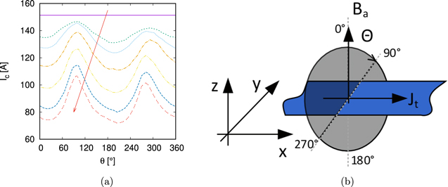
Figure 2. (a) The Ic(B, θ) measured data on a 4 mm wide SuperOx tape for the applied fields Ba = 0, 36, 49, 72, 100, 144, 180 mT in the arrow direction, using the set-up in Bratislava [44]. (b) Sketch of the Ic(B, θ) measurements with the definition of the θ angle to the tape surface.
Download figure:
Standard image High-resolution imageUnless stated otherwise, the number of elements in the superconductor are 15 × 15 × 9 per tape, with the last the number of elements in the thickness. We have checked that with this mesh, the calculated cross-field demagnetization is mesh independent. As can be seen in figure 3, the difference in trapped field in one tape for both at the end of relaxation and after 10 cycles is the same for 7 and 9 cells across the thickness. We also checked that the results are insensitive to the number of cells in the tape width and, being this the mesh used for the comparison with experiments. For all calculations, we use a tolerance for J of 0.01% of Jc at zero magnetic field, although we checked that the results do not differ for a tolerance of 0.001%.
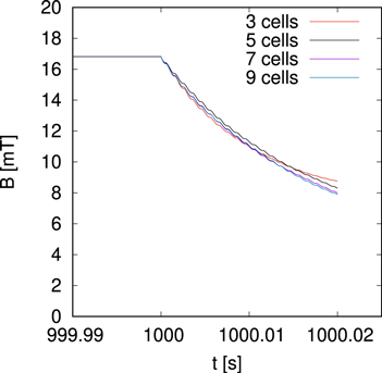
Figure 3. The modeling results of cross-field demagnetization are mesh independent for the mesh of 15 × 15 × 9 elements used in each tape. Results above are for a single tape with several numbers of cells in the thickness with ripple field of 240 mT amplitude and 500 Hz frequency, 10 cycles of ripple field, and the FC process shown in figure 9 followed by 900 s of relaxation. Cross-field demagnetization starts at 1000 s.
Download figure:
Standard image High-resolution imageThe variational formulation of MEMEP has been extended to take magnetic materials into account, as shown in the 2D examples of [45]. However, magnetic materials are not yet implemented in the 3D version of the software. This is not an issue in this article because the studied tape substrate is non-magnetic.
3.3. 3D FEM model
Here, we use FEM in order to benchmark the MEMEP 3D method. The FEM model is based on the H-formulation of Maxwell's equations implemented in the finite element program COMSOL Multiphysics [46]. Due to the necessity of simulating the air between and around the SC tapes typical of the FEM approach, care had to be taken in building the domains and the mesh. In order to avoid an excessive number of degrees of freedom, an approach based on sweeping a 2D geometry and mesh was followed (see figure 1 of [32] for an example). The external magnetic field was applied on the boundary of the air domains by means of Dirichlet boundary conditions. A magnetic field of Bz = 300 mT was assigned to all simulated domains as an initial condition. For FEM, we use 15 × 15 × 5 elements in each SC tape and a tolerance of 0.5%.
4. Results and discussion
There is a widespread effort to fully understand the cross-field demagnetization process. However, most studies have found only qualitative agreement with measurements. We focused on 3D modeling with all finite size effects, and hence the results can be compared with measurements on short samples. For the comparison to experiments, the model assumes the real dimensions of the measured sample and measured Jc(B, θ) dependence. Before comparing to experiments, we analyze the influence of several parameters like the SC layer thickness and gap between tapes. For this analysis, we study first the magnetization process and later the cross-field demagnetization.
4.1. In-plane magnetization of single tape with variation of thickness
The first study is about in-plane magnetization due to a parallel applied magnetic field. A sketch of the modeling case and the dimensions is shown in the figure 4. The magnetization loop is calculated only for the Mx component, because the applied magnetic field (of amplitude 50 mT and 50 Hz frequency) is along the x axis. We used a thicknesses of the SC layer d in the range from 1–1000 μm for this case. We assume constant Jcd, with Jc = 2.72 × 10¹⁰ A m−2 for d = 1 μm and an n power law exponent of 30.
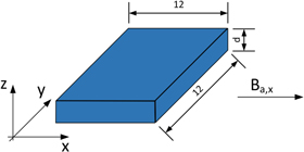
Figure 4. Single SC tape for the thickness dependence study (d = 1, 10, 100, and 1000 μm). Dimensions in the sketch are in millimeters.
Download figure:
Standard image High-resolution imageThe magnetization increases with tape thickness (figure 5(a)). This is not the case for the CSM, which we approximate as a power law with exponent n = 200 (figure 5(a)). All magnetization loops for different thickness are within 2%, without being identical due to the finite power law exponent (figure 5(b)). However, commercial SC tapes have an n value of around 30 in the self-field. The thickness dependence is due to higher electric fields from the applied magnetic field in thicker tapes. The relatively low n value of 30 allows J > Jc for high local electric fields, and hence the magnetization increases with thickness roughly as 14% for each increase in thickness by a factor 10. This effect does not appear for the CSM, since  is limited to Jc, irrespective to the value of the non-zero electric field. Therefore, we can already see that the sample thickness plays a role in the response to the ripple field. The effects of the thickness are much more important for the cross-field demagnetization (section 4.2), which is also significant for the CSM [27, 47]. In the calculations in the following sections, we assume the real thickness of 1.5 μm for comparison to experiments and 10 μm for the purely numerical analysis.

Figure 5. The magnetization loops Mx of a single tape increase with thicknesses d = (1, 10, 100, 1000 μm), while keeping the sheet's critical current density Jcd constant. The model assumes a realistic n power law exponent (a) n = 30 and a situation close to the critical state model (b) n = 200.
Download figure:
Standard image High-resolution image4.2. Cross-field demagnetization of one tape with variation of thickness
Next, we present a more detailed study about thickness influence for the cross-field demagnetization. The model assumes a single tape with thicknesses from 1–100 μm. Here, we make a similar analysis as for the published 2D modeling starting from 10 μm upwards for a single cycle [5] but now for the 3D configuration, starting from 1 μm, and up to 10 cycles, being more relevant for experiments. Now, the critical current density is inversely proportional to the thickness. The Jc of 1 μm tape is Jc = 2.72 × 10¹⁰ A m−2 and the n value is 30. The tape is magnetized with the perpendicular applied field to the tape surface by the FC method. The field is ramped down with rate 30 mT/s over 100 s with following relaxation of 900 s. Afterwards, a sinusoidal transverse field of 500 Hz is applied along the x axis.
The demagnetization rate greately increases with the thickness (figure 6), even though Jc is inversely proportional to the thickness. The clear thickness dependence shows the importance of the sample thickness, being even more relevant than in section 4.1. Therefore, the thickness in the model is very important for the cross-field demagnetization, where ripples are in the in-plane direction. The model cannot assume thicker films and lower proportionally the critical current density, as already predicted by Campbell et al [25]. Since the SC layer in most ReBCO tapes is of the order of 1 μm, 3D modeling is very challenging due to the high aspect ratio. Most previous works, which are in 2D, assumed unrealistically thicker samples due to numerical issues.
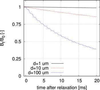
Figure 6. For constant Jcd, with d being the tape thickness, the trapped field, Bt, decreases with the thickness, and hence the model needs to take the real tape thickness of the order of 1 μm into account. Calculations in this graph are for 1 mm above a single tape, power law exponent n = 30, and normalized to the trapped field at the end of relaxation, B0.
Download figure:
Standard image High-resolution image4.3. Trapped magnetic field in the stack of tapes
The next study is about the influence of number of tapes and gap between SC layers in the stack on the initial trapped field. We used the same geometrical parameters as in section 4.1. The SC layer is 10 μm thick with Jc = 2.72 × 10⁹ A m−2 and n = 30. As shown above, it is not possible to take a larger superconductor thickness and a proportionally lower Jc for cross-field demagnetization and the transverse applied field. However, this simplification can be made for applied fields perpendicular to the tapes [48, 49]. The cause is that the electric field due to the applied magnetic field is roughly uniform in tape thickness and the effect of the self-magnetic field can be averaged over the tape thickness.
The stack is magnetized by the FC method along the z axis. The initial applied magnetic field is 1 T with a ramp down rate of 10 mT/s, because the perpendicular penetration field Bp of one tape is 27.2 mT. Afterwards, we leave a relaxation time of 900 s, which is long enough to reach the stable state of the trapped field. The trapped field decreases logarithmically during relaxation, and hence after a short time the reduction is almost negligible. The trapped field is calculated 1 mm above the top tape, similar to a Hall probe experiment. The probe position is more relevant for commercial application than the magnetic field in the tape or between the tapes. The sketch of the modeling case is shown in figure 7(a).
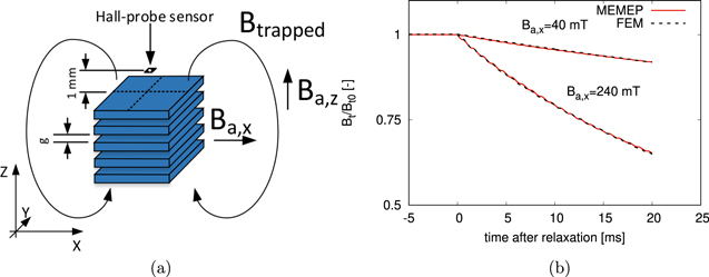
Figure 7. (a) Stack of five tapes with a Hall probe position and the direction of the magnetization and demagnetization fields Ba,z and Ba,x, respectively. The gap between the SC layers is 200 μm. (b) The cross-field demagnetization of a two-tape stack calculated by the MEMEP 3D method and the FEM. The methods are in very good agreement for both cross-field amplitudes 40 and 240 mT.
Download figure:
Standard image High-resolution imageThe trapped field increases with the number of tapes as shown in figure 8. The big gap of 200 μm between the SC layers causes saturation of the trapped field. The trapped field decreases with the gap g, and hence SC tapes with thinner Hastelloy, stabilization, and any additional isolating layers are more suitable for applications based on stacks of tapes. The cause of the decrease in the trapped field with increasing the gap is the increase of the overall thickness-to-width ratio, since the contribution of the bottom tapes to the trapped field on the top decreases with the overall thickness. This decay with the thickness is faster in 3D calculations than in cross-sectional 2D. The cause is that in short tapes the magnetic field created by closed loops are dominated by the dipolar term and decays with the distance r as  , while in 2D the decay is 1/r2.
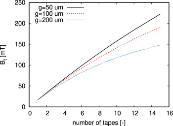
Figure 8. The trapped field increases with the number of the tapes in the stack but decreases with the gap, g, between SC layers.
Download figure:
Standard image High-resolution image4.4. Benchmark of the MEMEP 3D method with the FEM
Next, we cross-check the MEMEP 3D method and the FEM. The comparison case is for a two-tape stack only, for simplicity. The SC layer is 10 μm thin with a 200 μm gap between the layers. The electrical parameters are the same as Jc = 2.72 × 10⁹ A m−2 and n = 30. The mesh contains 15 × 15 × 5 cells per SC layer. The computing time for this mesh and the cross-field of 240 mT is 3–4 h for the MEMEP 3D method and 14–15 h for the FEM. MEMEP used a computer with i7-4771 CPU at 3.5 GHz and the FEM used a workstation with i7-4960X CPU at 3.60 GHz.
The magnetic moment of the sample at the end of relaxation differs only by 4% between both models. Therefore, the screening current calculations are in very good agreement.
The result of the trapped field 1 mm above the top surface is shown in figure 7(b). The trapped field is normalized by the trapped field at the end of the relaxation time, B0. The value of B0 is 32.4 mT for the MEMEP 3D method and 28.6 mT for the FEM. The comparison is in good agreement, even though the trapped field has an 11% difference This difference is due to inaccuracies in the trapped magnetic field by the FEM, due to the relatively coarse mesh in the surrounding air. This could also be the cause of the discrepancy in the magnetic moment. Nevertheless, the demagnetization rate is the same for both methods. This confirms the validity of the MEMEP 3D calculations, being more accurate than FEM for this configuration.
4.5. Cross-field demagnetization for high speed rotating machines (500 Hz)
The next study is about the entire cross-field demagnetization process in the stack of five tapes. A sketch of the modeling case is shown in figure 7(a) and it uses the same parameters as in the previous sections. The gap g between the SC layers is 200 μm and the SC layer is 10 μm thick. The time evolution of the magnetizing field, Baz, and the trapped field on the stack, Bt, are shown in figure 9. At 1000 s, the sinusoidal ripple field, Bax, of 500 Hz is switched on.
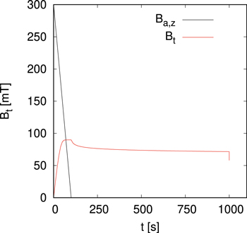
Figure 9. Time evolution of the magnetizing applied field, Ba,z, and the trapped field, Bt, on the stack. FC magnetization and subsequent end of relaxation are at 100 and 1000 s, respectively. Afterwards, the stack experiences cross-field demagnetization.
Download figure:
Standard image High-resolution imageThe study of the current density inside the stack is on the x and y cross-section planes, as defined in figure 10. The current density maps (figure 11) are in real scale except the z coordinate. Since the tapes are 10 μm thick and the gap is 200 μm wide, the variations in the thickness of the current density are not visible in the real scale. Therefore, the map contains the real data, but the SC cells are shown with the same height as the the gap cells. Since we use an odd number of cells in the x and y directions, there appears a central cell with zero current density in figures 11(a), (d)–(f), causing the vertical purple line. The study case is with a cross-field amplitude 240 mT.
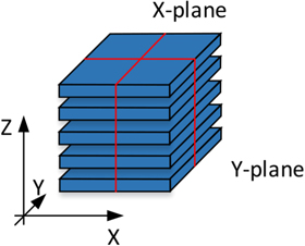
Figure 10. The cross-sectional planes are at x = 6 mm and y = 6 mm for the current density color maps.
Download figure:
Standard image High-resolution image
Figure 11. 3D current density color maps during cross-field demagnetization. The perpendicular component of the current density in the cross-sections at the middle of the stack at x = 6 mm, y = 6 mm, (a), (d) after 15 min of relaxation (b), (e) at the first positive peak of ripple field 240 mT (c), (f) at the last positive peak (10th cycle). The air and the SC cells are plotted on the color maps with the same height for better visibility. However, the calculation uses the real dimensions of the sample.
Download figure:
Standard image High-resolution imageThe stack at the end of the relaxation is fully saturated with Jx ≈ Jc and Jy ≈ Jc as shown in figures 11(a) and (d), respectively. The Jz component is very small, around 0.001Jc due to the thin film shape. The current density magnitude is below the critical current density Jc, because of flux relaxation.
The applied cross-field at the first positive peak causes small penetration of the screening current from the top and bottom of each individual tape, as can be seen in figure 11(b). The penetration front on the y-plane rewrites the remanent state of the current density Jy to the positive sign from the top and with a negative sign from the bottom of each tape (figure 11(b)). This process can be explained by the Bean model of the infinite thin strip [27] or other numerical 2D modeling [5, 25]. In our stack, the penetration front contains both the Jy and Jz components, even though Jz is very small. The x-plane section of figures 11(d)–(f) shows that the Jx current density from remanent state progressively decreases at each cycle due to the effect of Jy (and also Jz in a lesser amount) caused by the ripple field, which penetrates from the top and bottom of each individual tape. This is the same qualitative behavior found for SC bulks [30]. The oscillations in the current profiles in figures 11(e) and (f) are due to a numerical error.
Finally, we study in detail the current density maps at the tenth positive peak of the cross-field. At the y-plane, the Jy current density component penetrates slightly more than after the end of the first cycle. The penetration depth is 2 cells from the top and bottom of each layer within the total of 9 cells per SC layer (figure 11(c)). The lowest penetration is in the inner tapes. The cause is that the inductive coupling with the rest of the tapes is the largest. This enhanced inductive coupling slows down the demagnetization decay due to the dynamic magneto-resistance [27, 47], with exponential decay for a large enough time. At the x-plane, the Jx component is almost completely concentrated in three cells in the center of each SC layer (figure 11(f)). The current maps show the slow penetration of the current front and the erasing process of the remnant state with increasing the number of cycles. Although Jz plays a role in the cross-field demagnetization, its value is much below Jc, and hence reducing Jc in the z direction will not cause any significant change.
The trapped magnetic field Bt during the whole process is calculated 1 mm above the top surface (figure 9). After relaxation, we applied cross-fields with two different amplitudes, 40 and 240 mT, in order to see the behavior in the fields below and above the penetration field Bp of the stack. The parallel penetration field Bp,∥ of 1 tape is 17 mT according to the slab CSM [50, 51],

The demagnetization rate for the 40 mT cross-field is very low, with a 3.9% drop of the trapped field after ten cycles (figure 12). The higher cross-field of 240 mT makes a 19.1% reduction of the trapped field. The roughly linear demagnetization is consistent with Brandt's predictions, where there is linear decay for the first few cycles [27]. However, the method of [27] is based on the Bean model and for a single tape. For applied fields above the penetration field, as is the case of both 40 and 240 mT, demagnetization will continue until the entire sample is demagnetized.
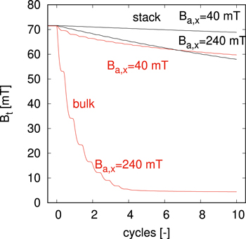
Figure 12. The cross-field demagnetization of the trapped field, Bt of the studied stack of tapes demagnetizes slower than its equivalent bulk (sketch in figure 14). Calculations for transverse field amplitudes of 40 and 240 mT with 500 Hz frequency.
Download figure:
Standard image High-resolution imageFor high demagnetization rates, such as high ripple field amplitudes or thick SC layers, we observe steps in the demagnetization of the time evolution (figures 6 and 12). These steps are also present in bulks (see figure 12 and reference [30]) and are due to the changes in the rate of current density penetration within an AC cycle. Current penetration from the top and bottom layers of each tape slows down at the AC peaks, causing a plateau in the trapped field.
A more detailed trapped field profile is calculated along the (red) "Bt" line above the sample shown in figure 13(a). The profile has the usual symmetric peak at the end of the relaxation time (figure 13(b) black curve). The first positive peak of the cross-field of 240 mT makes a small reduction of the trapped field (figure 13(b) blue curve), since the current density has not changed significantly due to the transverse field. The last positive peak of the cross-field is shown in figure 13(b) as a red line. The trapped field peak is always symmetric without any shift, contrary to cubic bulk samples [30]. The cause of this difference is the thin film shape of the tapes, as follows. For the bulk, the trapped field depends on the current distribution across the thickness, with a higher contribution for J closer to the top surface. Since J does not have mirror symmetry toward the yz-plane, (only inversion symmetry toward the bulk center) the trapped field on the surface is not symmetric. In contrast, the trapped field in the thin films only depends on the average J across the tape thickness, with variations of this dimension being irrelevant. Since the average thickness of J does have mirror symmetry with respect to the yz-plane for each tape of the stack, the trapped field on the surface also presents this mirror symmetry.
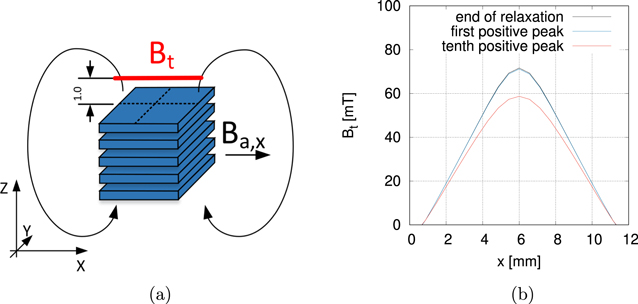
Figure 13. (a) The position of the calculated trapped field profile Bt is 1 mm above the stack. (b) The trapped field profile decreases during demagnetization by Ba,x with an amplitude of 240 mT and 500 Hz.
Download figure:
Standard image High-resolution image4.6. Comparison of cross-field demagnetization in a stack of tapes and bulk
There are two alternatives for high temperature supermagnets: stacks of tapes and bulks. Both candidates broke the world record of a trapped field, at above 17 T with slightly higher values for the stack [1, 2]. However, both behave differently under cross-fields. Therefore, we performed a short simple comparison between them. We used the same geometry for the five-tape stack as was mentioned above. We calculated the engineering current density for the stack Jce = 160 MA m−2 and set it as critical current density Jc for the bulk. The samples with their size dimensions are shown in figure 14. We estimated the parallel penetration field of the equivalent bulk from the slab approximation

with dall = 0.85 mm of the overall stack thickness and  mT.
mT.
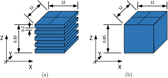
Figure 14. Bulk and stack of tapes with the same geometrical dimensions and engineering critical current density for comparison. Dimensions are in millimeters.
Download figure:
Standard image High-resolution imageThe trapped field at 1 mm above the top surface at the end of the relaxation time of 900 s is similar for the stack (71.6 mT) and the bulk (71.4 mT), because of similar parameters. The end of the relaxation time is marked as the 0 cycle in figure 12. The bulk shows a significant drop in the trapped field of around 93% in the first four cycles of the 240 mT cross-field, larger than the bulk penetration field (85 mT). In the case of low cross-field amplitude of 40 mT, the drop is around 16%. For a large number of cycles, the trapped field will decrease until a quasi-stable state is reached, because the ripple field amplitude is below the parallel penetration field of the bulk [27], with the latter dominated by a slow flux creep decay [52]. The stack shows a much slower demagnetization rate for the high cross-field of 240 mT and the trapped field drop in ten cycles is only 19%. The same behavior is observed for the low cross-field of 40 mT with a very low trapped field reduction of 3.9% at ten cycles. Nevertheless, demagnetization should continue until it completely demagnetizes the sample, because the ripple field is above the parallel penetration field of one tape (17mT). Therefore, for the high cross-field cases (ripple field above the parallel penetration field of the bulk) the stack of the tapes is more suitable. However, in the case of low fields the bulk is more suitable because the trapped field after many cycles reaches a non-zero asymptotic value. Nevertheless, if the super-magnet is submitted to a relatively low number of cycles, the stacks of the tapes are preferred in any case. Applications with low frequency ripples and built-in re-magnetization, such as certain low-speed motors and wind turbines, might also favor stacks of tapes, because of less re-magnetization.
4.7. Cross-field demagnetization: measurements and modeling
The last study is about measurements and comparison with calculations. The stack consists of five tapes and the parameters are listed in the table 1. The details about the sample and the measurements are given in section 2. The measurements are performed for two cross-field frequencies: 1 and 10 Hz.
Table 1. Input parameters of the measurements and calculation.
| Size [mm] | 12 × 12 × 0.001 5 |
|---|---|
 [A/m2] [A/m2] |
2.38 × 10¹⁰ |
 [T] [T] |
1.0 |
| Ramp rate [mT/s] | 10 |
| Relaxation [s] | 300 |
| Ec [V/m] | 1e-4 |
 [Hz] [Hz] |
0.1,1 |
| Bax [mT] | 50, 100, 150 |
| n [-] | 30 |
The demagnetization rate increases with the field (figure 15). The rate per cycle at low frequencies only slightly depends on the frequency, in agreement to [26]. The reason is that the higher frequency of the applied field causes a higher electric field, and hence the current density increases. This reduces both the penetration field and the demagnetization rate [30, 49, 53–55]. The measurements also show increased frequency dependence with field (figure 15). A possible cause might be the decrease of the power law exponent with the applied field amplitude (figure 16(a)). The oscillations observed in the measurements are most likely due to experimental noise.
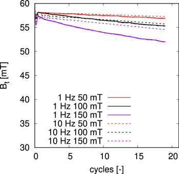
Figure 15. The measured demagnetization rate increases with the cross-field amplitude. There is also a low frequency dependence, although the demagnetization rate is similar for both frequencies.
Download figure:
Standard image High-resolution image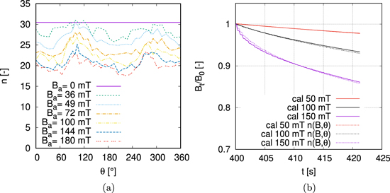
Figure 16. (a) The n(B, θ) measured data on a 4 mm wide SuperOx tape, measured in Bratislava by the set-up in [44]. (b) A comparison of the calculation with constant n = 30 and n(B, θ) dependence, both cases use Jc(B, θ) dependence. Using n(B, θ) slightly reduces the demagnetization rate for a few cycles, but later on it increases slightly.
Download figure:
Standard image High-resolution imageFor the model, we take three different assumptions for Jc: constant Jc; isotropic Jc(B), with B being the local modulus of the magnetic field; and anisotropic Jc(B, θ). Only the latest approach provides realistic predictions. The model uses a 1.5 μm thin SC layer with a 220 μm gap between them, with the rest of parameters the same as for the measurements listed in table 1.
The coarsest predictions are for constant Jc (figure 17). The measured Ic of the 12 mm wide SuperOx tape is 450 A at the self-field (or Jc = 2.5 × 10¹⁰ A m−2). We reduced Jc by 26% to the value Jc = 1.85 × 10¹⁰ A m−2, in order to get a similar trapped field, 58.9 mT, at the end of the relaxation time as the measurements, 58.1 mT. Naturally, this is an artificial correction of the stack self-field effect, and hence for constant Jc the predicting power is only in regard to the demagnetization rate. However, the predicted demagnetization rate is substantially lower than the measured one. The reason is that the assumed critical current density is too high, because of the missing Jc(B, θ) dependence in the model. The magnetic field reduces the critical current density, and hence it increases the demagnetization rate.
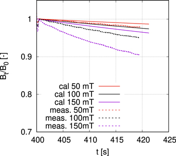
Figure 17. Comparison of the measurements and calculations (constant Jc = 1.85 × 10¹⁰ A m−2) of 1 Hz cross-field demagnetization. The constant Jc underestimates the demagnetization rate due to the missing Jc(B) dependence.
Download figure:
Standard image High-resolution imageAnother comparison between the model with Jc(B) dependence and measurements is shown in figure 18. The Jc(B) data was measured on the 4 mm wide SuperOx tape (figure 2). The critical current per tape width at the self-field for the measured tape (37.8 A/mm) is roughly the same as the 12 mm wide tape used in the stack (35.8 A/mm), with the latter value the minimum stated one by the producer. The theoretical difference is 5%, which is very small. The average tape Ic of the measured sample could be higher, around 440 or 450 A regarding typical deviations in SuperOx tapes, and hence even more close to that in the calculations. By now, we assume an isotropic Jc(B) dependence, taking the measured Jc(B, θ) values at perpendicular applied field. Then, we assume an isotropic angular dependence in the model. The cross-field is parallel to the tape surface, and hence the actual critical current density is larger than that in the model, also presenting lower reduction under magnetic fields than assumed. This is the reason why the demagnetization rate is overestimated for the high cross-fields of 100 and 150 mT.

Figure 18. Comparison of the measurements and calculations with the Jc(B) measured data of the 1 Hz cross-field. The Jc(B) dependence overestimates the demagnetization rate due to missing anisotropy dependence.
Download figure:
Standard image High-resolution imageThe last comparison here uses the measured Jc(B, θ) dependence. Now, the model agrees very well with the measurements (figure 19). The lowest deviation of the trapped field at the last cycle is 0.2% for 50 mT and 1.2% for the 100 mT cross-field. The highest cross-field amplitude causes the highest demagnetization in the calculation, with the difference of 4.0%. For low demagnetization, the demagnetization rate, β, is more relevant than the trapped field, which we can define as

with ti and tf the time at the beginning and end of the demagnetization process, respectively. For our configuration, which is similar to that in other works [5, 24, 25, 28], the error regarding this quantity is more strict than for the trapped field (table 2), resulting in errors below 20% for ripple fields of 100 mT or below.

Figure 19. A comparison of the measurements and calculations with the  measured data of the 1 Hz transverse field. The calculation agrees very well for the low cross-field up to 50 mT. The cross-field above 50 mT requires Jc(B, θ) measured data with a parallel component to the current path. However, the results for higher fields are of good accuracy of around 4%.
Download figure:
Standard image High-resolution imageTable 2.
Deviation of the MEMEP 3D modeling results of the trapped field, Bt, and the demagnetization rate defined as ![$[{B}_{t}({t}_{{\rm{i}}})-{B}_{t}({t}_{{\rm{f}}})]/({t}_{{\rm{f}}}-{t}_{{\rm{i}}})$](https://content.cld.iop.org/journals/0953-2048/33/4/044019/revision2/sustab5acaieqn15.gif) , with ti and tf the time at the beginning and end of the demagnetization process, respectively. The second error estimation is more strict for low demagnetization rates. The results are for the 20th cycle of the configuration and are shown in figure 19.
, with ti and tf the time at the beginning and end of the demagnetization process, respectively. The second error estimation is more strict for low demagnetization rates. The results are for the 20th cycle of the configuration and are shown in figure 19.
| Ripple field amplitude [mT] | 50 | 100 | 150 |
|---|---|---|---|
| Deviation of trapped field [%] | 0.2 | 1.2 | 4.0 |
| Deviation of demagnetization rate [%] | 3.0 | 19 | 29 |
We also study the effect of the measured n(B, θ) dependence (figure 16(a)) compared to the constant n = 30 assumption. The demagnetization rate is only slightly changed with n(B, θ) dependence (figure 16(b)). The local J increases with decreasing the n value, and hence it changes the demagnetization rate. There is a slight reduction of the demagnetization rate at the first few cross-field cycles. However, later on the demagnetization rate overlaps with the constant n curve and slightly increases. The demagnetization rate is more influenced by n(B, θ) for cross-fields above 50 mT.
There are several reasons for the reduction in the accuracy of the model. The Jc(B, θ) data covers correctly only the Jc in the y-plane position (figure 10), where the current is perpendicular to the magnetic field. However, at the x-plane, the current density presents a large component parallel to the applied magnetic field in the x direction. This is the so-called force-free configuration [35], where Jc should be different than the typical Jc(B, θ) measurements with  always perpendicular to the transport direction. Since measurements show that Jc in force-free configuration is often higher [56, 57], this could explain the overestimated cross-field demagnetization in the model. Measurements of solid angle dependence, Jc(B, θ, ϕ) with ϕ the angle of
  with the current density, are scarce for any type of sample [56] and missing for this particular tape. The cause is the complexity of the measurements, requiring a double goniometer [58–61]. The model uses Jc(B, θ) data for both components Jx and Jy, and hence there is a discrepancy between the model and the real measurements in the highest cross-fields. The discrepancy between the measurements and calculations could also be due to variations in the magnetic field dependence of Jc between the measured one and the SuperOx tapes in the stack.
4.8. Error caused by 2D modeling assumptions
Finally, we check the relevance of 3D modeling, in contrast to cross-sectional 2D computations. Since this is entirely a geometrical effect, the constant Jc assumption is sufficient. For the calculations, we use the same conditions as those in the previous section, about comparison to experiments.
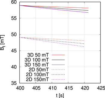
As can be seen in figure 20, the trapped field for 2D modeling is around 20% lower at the end of the relaxation (400 s). In addition, there are also substantial differences in the relative demagnetization rate, as defined in equation (3). 2D modeling predicts a fasterdemagnetization rate by 33%, 35%, and 39% for 50, 100, and 150 mT ripple field amplitudes, respectively, as calculated for the 20th cycle. This will worsen the agreement with experiments, where the 3D model already overestimates the demagnetization rate for 100 and 150 mT, possibly caused by neglecting force-free effects. Since 2D modeling also inherently neglects force-free effects, geometrical and force-free errors accumulate, which might cause a deviation as large as 60% for the 20th cycle and high ripple fields.
Figure 20. Using the infinitely long assumption (2D modeling) incurs around a 20% error in the trapped field, Bt, and a higher demagnetization rate. 2D modeling also disables the possibility of taking force-free effects into account, as well as studying the parallel component of  to the ripple field.
Download figure:
Standard image High-resolution image
In addition, 2D modeling cannot study the parallel component of  to the ripple field. This component, the x component in figures 10 and 11, has roughly the same contribution to the trapped field as the y component, the latter being the only one computed in 2D modeling. 2D modeling also disables the possibility to take force-free effects into account, potentially incurring to further errors.
5. Conclusions
This article presents 3D modeling of cross-field demagnetization in stacks of ReBCO tapes for the first time, and this is a substantial achievement according to the methodology in [31]. This 3D modeling enables taking the sample end effects into account, being essential in laboratory experiments, usually made of square tapes, and certain applications, such as axial flux motors or nuclear magnetic resonance magnets. The 3D geometry and the MEMEP 3D model used also enable taking force-free effects (or also ab axis anisotropy) into account, as a possible cause of disagreement with the experiments at high ripple fields.
The studied shape, modeled by the MEMEP 3D method, is very challenging, since we need to keep the real superconductor thickness, of the order of 1 μm, and mesh the layer across its thickness, achieving cells in the range of 100 nm. This results in an aspect ratio of the 3D cells of around 5000. The MEMEP 3D modeling tool showed the full cross-field demagnetization process in a five ReBCO tape stack and the 3D screening current path. This also enables studying the current component parallel to the ripple field, in contrast to 2D modeling, which can describe the perpendicular component only.
In this article, we present a complete study of cross-field demagnetization by 3D modeling. Among other issues, we confirm the need for the real thickness of the tape, around 1 μm, by 3D modeling up to ten cycles. When comparing the stack with the equivalent bulk, the stack demagnetizes slower. However, we expect that the bulk reaches a stable state without a further drop in the trapped field under cross-fields lower than the bulk penetration field.
The measurements of the five tapes stack assembled from 12 mm wide SuperOx tapes showed an increased demagnetization rate with the cross-field. A comparison with the calculations revealed that the constant Jc and isotropic Jc(B) dependences are not sufficient for cross-field modeling, and Jc(B, θ) dependence is necessary. The MEMEP 3D calculations agree with the measurements. Although the accuracy is very high regarding the total trapped field (around 4% is the worst of the cases), the demagnetization rate presents deviations as high as 29%. To improve the predictions at higher applied fields, it might be necessary to take the full solid angle dependence, Jc(B, θ, ϕ), into account, which includes macroscopic force-free effects. The n(B, θ) dependence showed only a slight influence on the demagnetization rate.
The results in this article indicate that the 2D assumption causes a higher error in the demagnetization rate, as defined in equation (3), than the expected deviation from neglecting force-free effects for all ripple field amplitudes. However, for high ripple fields, both features produce a comparable error. Since 2D modeling also inherently neglects force-free effects, both errors accumulate, which might cause an error as large as 60% (at the 20th cycle and large ripple fields).
In conclusion, we have shown that 3D modeling can qualitatively predict cross-field demagnetization in stacks of tapes, contrary to previous 2D modeling. This qualitative study has been possible thanks to the computing efficiency and parallelization of the MEMEP 3D method. The analysis here suggests that force-free effects may be important in the measured samples, pointing out the interest of Jc(B, θ, ϕ) measurements over the whole solid angle range.
Acknowledgments
We acknowledge M Vojenčiak for the critical current and power law exponent measurements and A Patel for discussions. The authors acknowledge the financial support of the European Union's Horizon 2020 research innovation program under Grant Agreement No. 7231119 (ASuMED consortium). M K and E P acknowledge the use of computing resources provided by the project SIVVP, ITMS 26230120002 supported by the Research & Development Operational Programme funded by the ERDF, the financial support of the Grant Agency of the Ministry of Education of the Slovak Republic and the Slovak Academy of Sciences (VEGA) under Contract No. 2/0097/18, and the support of the Slovak Research and Development Agency under Contract No. APVV-14-0438.