
Abstract
2D lattices are widely popular in micro-architected metamaterial design as they are easy to manufacture and provide lightweight multifunctional properties. The mechanical properties of such lattice structures are predominantly an intrinsic geometric function of the microstructural topology, which are generally referred to as passive metamaterials since there is no possibility to alter the properties after manufacturing if the application requirement changes. A few studies have been conducted recently to show that the active modulation of elastic properties is possible in piezoelectric hybrid lattice structures, wherein the major drawback is that complicated electrical circuits are required to be physically attached to the micro-beams. This paper proposes a novel hybrid lattice structure by incorporating magnetostrictive patches that allow contactless active modulation of Young's modulus and Poisson's ratio as per real-time demands. We have presented closed-form expressions of the elastic properties based on a bottom-up approach considering both axial and bending deformations at the unit cell level. The generic expressions can be used for different configurations (both unimorph or bimorph) and unit cell topologies under variable vertical or horizontal magnetic field intensity. The study reveals that extreme on-demand contactless modulation including sign reversal of Young's modulus and Poisson's ratio (such as auxetic behavior in a structurally non-auxetic configuration, or vice-versa) is achievable by controlling the magnetic field remotely. Orders of difference in the magnitude of Young's modulus can be realized actively in the metamaterial, which necessarily means that the same material can behave both like a soft polymer or a stiff metal depending on the functional demands. The new class of active mechanical metamaterials proposed in this article will bring about a wide variety of design and application paradigms in the field of functional materials and structures.
Export citation and abstract BibTeX RIS

Original content from this work may be used under the terms of the Creative Commons Attribution 4.0 license. Any further distribution of this work must maintain attribution to the author(s) and the title of the work, journal citation and DOI.
1. Introduction
The microstructural geometry of 2D lattices plays a vital role in determining the mechanical properties of the entire structure, and such systems can be constructed by repeating a unit cell periodically. Over the past few years, various shapes and topologies (triangular, Kagome, hexagonal, N-Kagome, foam structures, origami, star-shaped, chiral, square and other tailor-made geometries) of such lattice structures have been studied to understand the variation in the effective mechanical properties as the microstructure of the lattice changes (Lakes 1987, Grima et al 2000, Song et al 2008, Zhang et al 2008, Schenk and Guest 2013, Bückmann et al 2014, Shan et al 2015, Li et al 2019, Bacigalupo and Gambarotta 2020, Wei et al 2020, Huang et al 2021, Qi et al 2021, Xu et al 2021). These artificially engineered metastructures (often referred to as metamaterials) have a wide range of applications in the field of vibration and wave propagation, multi-functional modulation of static deformations, impact resistance, indentation, stability control and programmable shape modulation (Fleck et al 2010, Mukhopadhyay et al 2019, Du et al 2021). In this paper, we deal with the contactless active modulation of elastic properties that in turn influence such applications.
Young's modulus and Poisson's ratio of lattice structures have gained significant attention from the scientific community since these properties play a central role in a range of aforementioned mechanical applications. Recent studies have concluded that few geometries exhibit positive, negative, and zero Poisson's ratios, including extreme values and mixed mode (Olympio and Gandhi 2010, Attard and Grima 2011, Gong et al 2015, Chen et al 2018, Huang et al 2018, Wang 2019, Gaal et al 2020, Wang et al 2020). The main drawback of such lattices is that the elastic properties are a function of only geometric entities; hence upon manufacturing, it is not possible to change them, and due to this, the application of such lattices is limited to passive applications only. Here, we provide a brief literature review of such passive lattices. Closed-form analytical expressions for equivalent elastic moduli of 2D planer cellular materials have been studied extensively as it is computationally efficient and provides necessary physical insights (Abd El-Sayed et al 1979, Zhang and Ashby 1992, Masters and Evans 1996, Gibson and Ashby 1999, Malek and Gibson 2015, Mancusi et al 2017). Different methodologies have been adopted to determine the elastic properties, i.e. considering only the bending deformation of the cell walls (Gibson and Ashby 1999, Singh et al 2021) and considering both axial and bending deformation of the cell walls (Adhikari et al 2020, Prajwal et al 2022, Singh et al 2022). Some of these works have also accounted for shear deformation, which is more effective in the case of thick-walled lattices with higher specific densities. For passive lattice structures, the elastic properties are an intrinsic function of geometric properties and it is widely known in hexagonal lattices that Poisson's ratio (Evans 1991, Harkati et al 2017, Srivastava and Bhattacharya 2020) is positive when the cell angle (refer to figure 1(b) for the definition of cell angle) is positive and negative when the cell angle is negative (auxetic structure). Recent studies in the area of passive lattice metamaterials include a novel concept of anti-curvature (Ghuku and Mukhopadhyay 2022), chiral, anti-chiral (Mousanezhad et al 2016) and various hierarchical microstructures (Kagome honeycomb, Kagome honeycomb triangular, Hierarchical re-entrant honeycomb, Double arrow head) (Wang et al 2021, Dudek et al 2022, Xu et al 2022, Zhan et al 2022, Zhang et al 2022), 3D lattices with multi-directional auxeticity (Mukhopadhyay and Kundu 2022) and multi-material microstructures (Mukhopadhyay et al 2020).
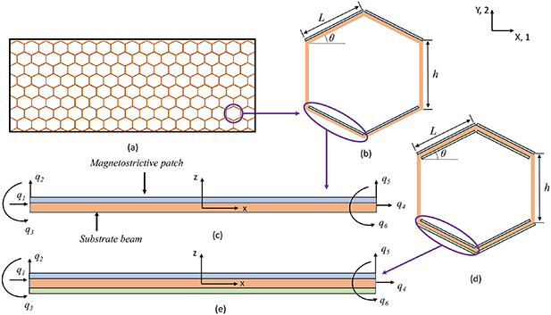
Figure 1. Magnetostrictive lattice microstructures for contactless active modulation. (a) The representation of honeycomb lattice structure in the X–Y (or 1–2) plane. (b), (d) Detailed view of the unit cell of a hybrid honeycomb lattice (unimorph and bimorph configurations). (c), (e) The degrees of freedom (DOF) for the inclined cell wall (i.e. hybrid beam having unimorph and bimorph configurations) with magnetostrictive patch attached. Here, different colors in the bimorph beam (blue and green) represent the magnetostrictive patches having different material properties. Following a bottom-up framework, the stiffness matrix of the hybrid beam is used here to determine the deformation behavior of the unit cell. To derive the analytical formulation of the hybrid beam, a local coordinate system (x, z) has been taken, wherein the direction x is along the beam length. X, Y represent the global coordinate system. Here, q1, q2, q3 and q4, q5, q6 are the DOF at node 1 and node 2 respectively, which relate to u1, w1,  and u2, w2,
  .
.
Download figure:
Standard image High-resolution imageUnlike passive lattice metamaterials, as investigated in the majority of the literature in this field, the effective elastic properties of active lattice materials can be modulated as a function of external stimuli. In such hybrid (piezoelectric) lattice structures, the dependency of Young's modulus (E1, E2) and Poisson's ratio (ν12,  ) (Singh et al
2021, 2022) on voltage have been obtained in the literature by using two methodologies (considering only bending deformation, and considering both axial and bending deformations). It has been found that Poisson's ratios emerge to be a function of voltage only when both axial and bending deformations are considered, whereas Young's modulus is voltage-dependent in both the methodologies. In this context, Adhikari et al (2020) reported the uncommon negative values of transverse and longitudinal Young's modulus under dynamic conditions. Recent literature of Singh et al (2021, 2022)shows that negative Young's modulus is achievable under static conditions in piezoelectric lattices. However, the main drawback of the piezoelectric hybrid lattice structures is that numerous complex electric circuital connections need to be established to observe the desired effect. To overcome such lacuna, we propose simpler contactless multi-physical effects in lattice materials by applying a magnetic field and exploiting the magnetostrictive constitutive behavior of active materials.
) (Singh et al
2021, 2022) on voltage have been obtained in the literature by using two methodologies (considering only bending deformation, and considering both axial and bending deformations). It has been found that Poisson's ratios emerge to be a function of voltage only when both axial and bending deformations are considered, whereas Young's modulus is voltage-dependent in both the methodologies. In this context, Adhikari et al (2020) reported the uncommon negative values of transverse and longitudinal Young's modulus under dynamic conditions. Recent literature of Singh et al (2021, 2022)shows that negative Young's modulus is achievable under static conditions in piezoelectric lattices. However, the main drawback of the piezoelectric hybrid lattice structures is that numerous complex electric circuital connections need to be established to observe the desired effect. To overcome such lacuna, we propose simpler contactless multi-physical effects in lattice materials by applying a magnetic field and exploiting the magnetostrictive constitutive behavior of active materials.
The incorporation of magnetostrictive patches with passive substrate beams in lattice design can lead to extreme on-demand modulation of effective elastic properties in a contactless setup. Magnetostrictive materials, which we aim to use as an intrinsic material in the hybrid lattices, belong to the class of smart materials that show dimensional changes under the influence of a magnetic field and also depicts the converse effect of change in magnetization under the influence of externally applied stresses (Quandt and Seemann 1995, Bhattacharya and Murty 1996, Body et al 1997, Si and Cho 2004, Ghosh and Gopalakrishnan 2005, Chopra and Sirohi 2013, Sheikholeslami et al 2017, Xu and Shang 2019, Amiri et al 2020). Grima et al (2013) and Galea et al (2022) experimentally demonstrated the variation in mechanical properties by incorporating magnetic inserts/inclusions over the inclined cell walls of the lattice structure. Montgomery et al (2021) studied the modulation of attenuation band gap as externally applied magnetic field varies. In the current paper, a generalized unit cell-based formulation would be presented that can be adopted for different unimorph or bimorph configurations by including the effect of the axial and bending deformations. The capability of contactless on-demand modulation of Young's moduli and Poisson's ratios (including extreme attributes like sign-reversal) will be numerically demonstrated considering different microstructural configurations and the intensity of the external magnetic field. Hereafter in this paper, section 2 presents the modeling of the hybrid beam along with the validation against the available literature; section 3 presents the derived expressions for Young's modulus and the Poisson's ratio; section 4 of this paper provides critical insights into the active modulation of Poisson's ratios and Young's moduli; the concluding remarks have been presented in section 6.
2. Beam-level multi-physical deformation mechanics
2.1. Modeling of hybrid magnetostrictive beam
Hybrid beams comprised of a passive substrate and surface mounted magnetostrictive patch(es) with desired magnetostrictive constant (positive/negative as per the application requirement) are adopted as the elementary component of the active hybrid lattice, as shown in figure 1. The beams have been assumed to be Euler Bernoulli beam with the consideration of thin cell walls. The displacement of the hybrid beam in x–z plane can be represented as


From equations (1) and (2) we can write the strains in x and z directions as
The stress (Chopra and Sirohi 2013) in the substrate beam and the magnetostrictive patch (top and bottom) can be given as


Here, Ys and Ym are Young's modulus of the substrate beam and magnetostrictive patch, respectively. The magnetostrictive constant is d, and H is the applied magnetic field intensity.
The total potential energy of the hybrid beam can be given as the sum of the potential energy of the substrate beam and the magnetostrictive patch.
Substituting the equations from equations (4) and (5) in equation (6) we get
To derive a more general expression, total volume of the magnetostrictive patches can be written as the sum of top and bottom layers i.e. Vm
=  +
+  (here, b and t stand for top and bottom magnetostrictive films respectively). Equation (7) can be extended to equation (8) as
Here,  ,
,  ,
,  ,
,  are given as (for any point along the beam length)
Magnetic Energy (Xu and Shang 2019) can be given as
Taking the variational form of equations (8) and (10) we get

A two node beam element having three degrees of freedom (DOF) (i.e. axial, transverse and rotation) at each node has been considered with a scaled length of 1.


Taking variational of the above equations we get

Differentiating the above equations we get

where,

Shape functions are given by
Using the equations (13)–(18) and recalling them in order to solve further, we get
where,
Using Hamilton's principle and substituting the values from equations (12) and (19) in the following equation
Substituting the expressions from equations (12) and (19) in equation (21), the final form of equilibrium equation can be written as

the values of ![$[K]$](https://content.cld.iop.org/journals/0964-1726/31/12/125005/revision2/smsac9cacieqn10.gif) and
and  can be defined as
Subsequently, displacements of a beam due to change in the magnetic field intensity can be calculated by solving the following equation

The beams here (as a part of the lattice) have boundary condition of one end fixed. Accordingly, considering node 1 as fixed, we get that u1, w1 and  are equal to zero. The expressions of force vector {F} and stiffness matrix [K] are
the expressions of  ,
,  ,
,  and
and  are given as
the expressions of A, B and C are given as
the expressions of the dimensional constants like  ,
,  , As
,
, As
,  ,
,  , Hs
,
, Hs
,  ,
,  and Is
are discussed in the following subsection.
and Is
are discussed in the following subsection.
2.2. Determination of the beam constants
The constants used in the formulation provided in the preceding subsection are determined here. The detailed view showing the integration limits used to obtain the constants are taken from the neutral axis, which has been assumed to be at the center of the beam (refer to figure 2).
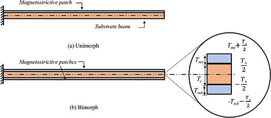
Figure 2. Mechanics of element-level magnetostrictive hybrid beams. Unimorph and bimorph configurations, having single and double magnetostrictive patches, respectively. The limits required to determine the constants for the unimorph and bimorph configurations have been marked from the geometric center as shown in (b).
Download figure:
Standard image High-resolution image2.2.1. Substrate beam.
Area of the beam is given as
First moment of area is given as
Second moment of area is given as
2.2.2. Magnetostrictive patch in unimorph configuration.
Area of magnetostrictive patch is given as
First moment of area is given as
Second moment of area is given as
2.2.3. Magnetostrictive patch in bimorph configuration.
Areas for top and bottom magnetostrictive patches are given as
First moment of areas for top and bottom magnetostrictive patches are given as
Second moment of areas for top and bottom magnetostrictive patches are given as
2.3. Validation of the proposed beam model
A cantilever beam is constructed by considering multiple layers of substrate material (as per the followed literature for validation), and on the top and bottom surface, magnetostrictive patches have been added. Note that we validate the beam-level formulation for a more generalized case of multi-layered substrates that will ensure the accuracy of isotropic single-layer substrate considered throughout the paper otherwise. The dimensions, ply angle and properties of the beam have been mentioned in table 1. The number of coil turns per unit length has been taken to be 20 000 turns m−1, and the static actuation has been analyzed at 1 A DC actuation coil current. The deflections obtained from the proposed model have been compared with the existing literature (Ghosh and Gopalakrishnan 2005), wherein the current results are found to be in good agreement as shown in table 2. As per descriptions in the followed literature for validation, the top magnetostrictive patch has been used as an actuator, whereas the bottom patch acts as a sensor. The values for Am and Hm in the force matrix have been taken from the unimorph configuration as the bottom patch is not contributing to the deformation of the hybrid beam.
Table 1. Details of the dimensions and material properties used to validate the current analytical framework. Dimensions and material properties (Ghosh and Gopalakrishnan 2005) of the substrate beam and the magnetostrictive patches used to validate the response of the multilayered hybrid beam with the existing literature.
| Parameter | Dimensions |
|---|---|
| Magnetostrictive patch length (m) | 0.5 |
| Magnetostrictive patch width (m) | 0.05 |
| Magnetostrictive patch thickness (m) |

|
| Magnetostrictive constant d (m A−1) |

|
| Young's modulus of magnetostrictive patch (N m−2) |

|
| Substrate beam length (m) | 0.5 |
| Substrate beam width (m) | 0.05 |
| Substrate beam thickness (m) |

|
Young's modulus of substrate beam ( in direction 1) (N m−2) in direction 1) (N m−2) |

|
Young's modulus of substrate beam ( in direction 2) (N m−2) in direction 2) (N m−2) |

|
| Shear modulus of substrate beam (G12) (N m−2) |

|
| Permeability in air (H m−1) |

|
Table 2. Beam-level validation of the current formulation with existing literature. The comparison of the tip displacement of hybrid beam obtained from the current formulation with existing literature. Here, the subscript represents the number of the substrate and magnetostrictive patches at the top\middle\bottom of the hybrid beam. The ply angle of the substrate beam has been kept equal to 0∘ and 90∘. We have taken such multi-layered configurations as per literature for the sake of validation.
| Ply sequence | Current formulation (mm) | Literature (mm) |
|---|---|---|
![$[m]/{[}0{]}_{10}/[m]$](https://content.cld.iop.org/journals/0964-1726/31/12/125005/revision2/smsac9cacieqn33.gif)
| 2.44 | 2.44 |
![$[m]/{[}90{]}_{10}/[m]$](https://content.cld.iop.org/journals/0964-1726/31/12/125005/revision2/smsac9cacieqn34.gif)
| 15.40 | 15.40 |
![${[}m{]}_{2}/{[}0{]}_{8}/{[}m{]}_{2}$](https://content.cld.iop.org/journals/0964-1726/31/12/125005/revision2/smsac9cacieqn35.gif)
| 6.97 | 6.97 |
![${[}m{]}_{2}/{[}90{]}_{8}/{[}m{]}_{2}$](https://content.cld.iop.org/journals/0964-1726/31/12/125005/revision2/smsac9cacieqn36.gif)
| 21.55 | 21.56 |
![${[}m{]}_{3}/{[}0{]}_{6}/{[}m{]}_{3}$](https://content.cld.iop.org/journals/0964-1726/31/12/125005/revision2/smsac9cacieqn37.gif)
| 14.38 | 14.39 |
![${[}m{]}_{3}/{[}90{]}_{6}/{[}m{]}_{3}$](https://content.cld.iop.org/journals/0964-1726/31/12/125005/revision2/smsac9cacieqn38.gif)
| 25.53 | 25.53 |
![${[}m{]}_{4}/{[}0{]}_{4}/{[}m{]}_{4}$](https://content.cld.iop.org/journals/0964-1726/31/12/125005/revision2/smsac9cacieqn39.gif)
| 23.41 | 23.41 |
![${[}m{]}_{4}/{[}90{]}_{4}/{[}m{]}_{4}$](https://content.cld.iop.org/journals/0964-1726/31/12/125005/revision2/smsac9cacieqn40.gif)
| 28.47 | 28.47 |
3. Derivation of lattice-level effective Young's moduli and Poisson's ratios
This section presents a general derivation applicable for both unimorph/bimorph cases under the influence of an external magnetic field and remote stresses applied to the lattice in the horizontal and vertical directions, respectively, as shown in figure 3. The derived expressions accommodate the variation in effective elastic properties of the lattice materials due to change in the external magnetic field. All the vertical cell walls contribute to the total deformation by axial deformation only; there is no possibility of bending deformation of the vertical cell walls in the symmetric unit cells as either the loading is parallel or perpendicular to these vertical cell walls. Moreover, to reduce the complexity of the problem the magnetostrictive patches have been applied to the inclined cell walls only. The displacement of the inclined cell walls has been categorized into two parts, axial and transverse (bending), which occur due to the application of externally applied magnetic field and mechanical stress. The axial and transverse displacements under the applied magnetic field and mechanical stress can be obtained with the help of stiffness matrix given in equation (28) by superimposing the deflections due to the forces from these two components, as shown in figure 5. The magnetic field for the inclined cell walls has been categorized into two parts: parallel to the inclined cell wall and perpendicular to the inclined cell wall. It should be noted that the components of the magnetic field, parallel and perpendicular to the unit cell, act in the opposite manner; i.e. if the magnetostrictive coefficient (d) is positive, the parallel component will try to extend the length of the cell wall whereas, the vertical component will try to reduce the length of the cell wall and vice versa. Hence, at a particular angle (45∘), there will be no influence of the magnetic field on the deformation of the unit cell.
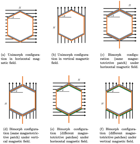
Figure 3. Configurations of honeycomb lattices under different magnetic fields. Unimorph/bimorph configurations under the application of magnetic field in horizontal and vertical direction. Here, blue and green colors represent different magnetostrictive materials. The arrows indicate the direction of the externally applied magnetic fields.
Download figure:
Standard image High-resolution imageDifferent configurations of the lattice structure shown in figure 3 deform as a combined effect of deformation under purely mechanical (Gibson and Ashby 1999) and purely magnetic loading (note that we consider only the elastic range of deformation here). The corresponding modes of deformations under pure mechanical stresses and pure magnetic fields are shown in figure 4. Note that the beam-level deformation curves will be opposite under opposite directions of mechanical far-field stress and magnetic field. Final shapes of the deformed configurations under the combined effect of magnetic field and mechanical stress can be obtained by adding the corresponding ordinates of the beam-level deformed shapes based on the intensity and directions of these two components.

Figure 4. Deformation of the lattice structure under combined loading. (a) and (b) show the deformation of the lattice structure when subjected to only externally applied stress in direction 1 and direction 2 respectively Gibson and Ashby (1999). The lattice structure having different configurations like unimorph bimorph (with same
 different magnetostrictive properties) will deform in a similar manner under magnetic field, as shown in subfigure (c) and (d). However, under the application of the magnetic field the magnitude of the deformation will vary, depending on various parameters like the direction and intensity of the externally applied magnetic field, properties of the magnetostrictive patch(es) and configuration of the honeycomb lattices. The resultant deformation under the combined effect of mechanical loading and magnetic field can be obtained by superimposing the displacements for the respective cases. Note that we have considered the lattice configurations in such as way that the deformation behavior of the two slant members are structurally symmetric.
Download figure:
Standard image High-resolution image3.1. Longitudinal Young's modulus E1 and Poisson's ratio 

The derivation for E1 and  are based on the free body diagram of the unit cell as shown in figure 5(a). For E1 , the external stress is applied in direction X (or 1) and the effective deformation of the unit cell is also obtained in the direction X (or 1). The magnetostrictive patch provides the additional force and moment (highlighted by the golden color in figure 5(a)) under the application of the magnetic field.

Figure 5. Deformation of a unit cell under remote mechanical stresses and magnetic field. (a) Deformation of the unit cell under the application of the externally applied stress (σ1) in X direction and applied magnetic field. The figure shows free-body diagram of the unit cell along with inclined cell walls, which have been used to determine E1 and  . (b) Deformation of the unit cell under the application of externally applied stress (σ2) in Y direction and applied magnetic field. The figure shows free-body diagram of the unit cell, which has been used to determine E2 and
  . Here, 1 and 2 represent the left and the right cell wall of the unit cell which can be made of the same or different material. The red color and golden color represent forces generated due to externally applied stress and magnetic field respectively.
Download figure:
Standard image High-resolution imageThe moment, M is given as
Axial and transverse displacements in general form under the influence of externally applied stress shown in figure 5(a) can be written as
the above mentioned expressions can also be represented as follows
here, t and b in the subscript represent the top and bottom magnetostrictive patches and i stands for 1, 2 that denote the left and the right cell wall of the unit cell. The expressions of P, R1, R2 and R3 are given as


where  ,
,  ,
,  ,
,  . Axial and transverse displacements in general form under the influence of externally applied magnetic field can be obtained from figure 5(a) and can be written as
the above mentioned expressions can also be represented as follows


where  . Total axial deflection under the combined loading of externally applied stress and magnetic field can be given as the sum of axial displacement due to applied magnetic field and externally applied stress.

Similarly, total transverse deflection under the combined loading of externally applied stress and magnetic field can be given as the sum of transverse displacement due to applied magnetic field and externally applied stress.

Displacement in direction 1 can be given as

Similarly, displacement in direction 2 can be given as

Subsequently the strain components are calculated as
Based on the definition of Young's modulus and Poisson's ratio, using the expressions of applied mechanical stress and strain components, we get the effective elastic properties as
The above mentioned formulation is generic; by using equations (60) and (61), E1 and  can be obtained for all the cases mentioned in figure 3. The major difference in all these cases is due to the variation in the parameters Am
, Hm
, Im
, d, Fm
and Mm
, which are different for different cases. Here, the dimensions for all magnetostrictive patches have been kept equal. However, the magneto-mechanical coupling coefficient is different for each beam. For deriving the numerical results later, the value of
can be obtained for all the cases mentioned in figure 3. The major difference in all these cases is due to the variation in the parameters Am
, Hm
, Im
, d, Fm
and Mm
, which are different for different cases. Here, the dimensions for all magnetostrictive patches have been kept equal. However, the magneto-mechanical coupling coefficient is different for each beam. For deriving the numerical results later, the value of  i.e. β has been kept equal to 2.5 and 4 whereas, the value of
  i.e. γ has been kept
  . The derived expressions are applicable for both horizontal and vertical magnetic fields. However, the effective values of H for each inclined unit cell under the influence of horizontal field and vertical magnetic field are
  and
and  respectively (considering the components along and perpendicular to the beam lengths).
3.2. Transverse Young's modulus E2 and Poisson's ratio

Stress σ2 is applied in direction Y (or 2) to derive the transverse Young's modulus E2, as shown in figure 5(b). The effective deformation of the unit cell is due to the combined effect of externally applied mechanical stress and magnetic field. It should be noted that as the loading is parallel to the vertical member, its axial deformation will contribute toward the overall displacement of the unit cell. Axial and transverse displacements in general form under the influence of externally applied mechanical stress in direction 2 can be given as
the above mentioned expressions can also be written as
here, the value of R1 is 1 as for the vertical member there is no magnetostrictive patch, i.e. αb and αt are zero.
Axial and transverse displacements in general form under the influence of externally applied magnetic field can be given as
the above mentioned expressions can also be written as
Total axial deflection under the combined loading of externally applied stress and magnetic field can be given as the sum of axial displacement due to applied magnetic field and externally applied stress

Total transverse deflection under the combined loading of externally applied stress and magnetic field can be given as the sum of transverse displacement due to applied magnetic field and externally applied stress


For all the cases the following deformation compatibility condition must be satisfied

where, 1, 2 stand for the left and right cell wall respectively. Further, from equilibrium we get

here, W1 and W2 can be obtained by solving equations (76) and (77). Moreover, the obtained expressions of W1 and W2 are different for different cases depending on the magnetostrictive and substrate beam properties.
Subsequently, the expressions of strain components can be obtained as
Based on the definition of Young's modulus and Poisson's ratio, using the expressions of global stress and strain components, we get
3.3. Remarks on unimorph and bimorph configurations
In this subsection, we present different possibilities for the placement of magnetostrictive patches in symmetric unimorph and bimorph configurations. It may be noted in this context that we have avoided the possibility of having asymmetric configurations here for the two slant members due to the additional complexity in derivation.
3.3.1. Case 1: symmetric unimorph.
In this case, we have same material on the left and right cell wall of the unit cell. The magnetostrictive patch is present on the top surface of the substrate beam only. Hence, substituting the parameters as  =
=  = 0,
= 0,  =
=  = 0,
= 0,  =
=  ,
,  =
=  ,
,  =
=  and
and  =
=  = Ys
, we get displacement of both the cell walls same i.e.
= Ys
, we get displacement of both the cell walls same i.e.  equals to
  .
.
3.3.2. Case 2: symmetric bimorph with same magnetostrictive patches.
In this case, we have the same material on the left and right cell wall of the unit cell. However, the material with same magnetostrictive coefficient has been used on the top and bottom surface of the substrate beam respectively, as shown in figures 3(a) and (d). Here, the parameters have been kept as  =
=  =
=  =
=  ,
,  =
=  =
=  =
=  ,
,  =
=  ,
,  =
=  and
and  =
=  = Ys
for both the cell walls (1 and 2), which make
= Ys
for both the cell walls (1 and 2), which make  equals to
  . This case is only valid when the value of
  ,
,  equals to 1 i.e. both top and bottom magnetostrictive patches are having same properties for both the slant beams. In this specific case, it can be observed that (when subjected to only externally applied magnetic field), only axial deformation of the slant members occurs.
3.3.3. Case 3: symmetric bimorph with different magnetostrictive patches.
In this case, we have different magnetostrictive patches on the top and bottom of the substrate beam, the same combination has been used over the left and right cell wall of the unit cell as shown in figures 3(b) and (e). When the lattice is subjected to combined loading of externally applied stress and magnetic field both axial and transverse deformation of the cell wall will take place. Here, the parameters have been kept as  =
=  =
=  =
=  ,
,  =
=  =
=  =
=  ,
,  =
=  ,
,  =
=  and
and  =
=  = Ys
which makes
= Ys
which makes  equals to
  . There can be three scenarios when the value of
  ,
,  has been kept (1) equal to −1 (special case), (2) any other negative value, or (3) any other positive value except 1. Here, the negative value of
  signifies that the top and bottom magnetostrictive patches are having magnetostrictive coefficients of opposite sign, whereas for the positive
  values both top and bottom patches can either have negative magnetostrictive coefficient or positive magnetostrictive coefficient. In the first sub case (when subjected to only externally applied magnetic field), the axial displacement will be zero and only transverse displacement will occur; however, in the later cases both axial and transverse displacement can be observed, when only magnetic field is applied.
3.4. Lattice-level validation of the current formulation
The formulation derived above has been validated with the existing literature for different possible cases considering passive lattice forms. The elementary beam level active deformation physics is validated separately in section 2.3. Such bi-level validation provides adequate confidence in the proposed computational framework.
3.4.1. Case 1: validation when axial deformation of the cell wall is neglected .
In this case, the cell walls have been assumed to be axially rigid. Moreover, there is no magnetostrictive patch on the substrate beam. In the derived expressions for the E1,  , E2 and
  substituting the value of the parameters as
  ,
,  , γs
,
, γs
,  ,
,  ,
,  ,
,  , H,
, H,  equals to zero and
  = Ys
in equations (60) and (61), equations (80) and (81) we get the following expressions given in equations (82) and (83), equations (84) and (85). These expressions exactly match with the formulae given by Gibson and Ashby (1999)
= Ys
in equations (60) and (61), equations (80) and (81) we get the following expressions given in equations (82) and (83), equations (84) and (85). These expressions exactly match with the formulae given by Gibson and Ashby (1999)
3.4.2. Case 2: validation when axial deformation of the cell wall is considered.
The expressions presented by Adhikari et al (2021) for the effective elastic moduli has been derived by considering both axial and bending deformations, but only applicable to conventional passive lattices structures. To validate the current expressions, we put the value of  ,
,  (as no magnetostrictive patch),
  (as the structure is symmetric) equals to zero and
  = Ys
in equations (60) and (61), equations (80) and (81) and the obtained expressions are given below in equations (86)–(89).
= Ys
in equations (60) and (61), equations (80) and (81) and the obtained expressions are given below in equations (86)–(89).
the above expressions exactly match with the formulae presented by Adhikari et al (2021), corroborating a lattice-level validation of the proposed computational framework.
4. Results and discussion
The formulation presented in the preceding sections is general, and it can be used for different configurations (unimorph or bimorph) along with different system parameters such as substrate material for the unit cell walls and properties of the magnetostrictive patches. However, for presenting numerical results here, the dimensions and the material property of the substrate beams have been kept the same. The realization of active variation in the effective elastic properties in a contactless manner has been reported here numerically for the first instance, which can be achieved under the combined influence of the externally applied mechanical stress and the magnetic field (refer to figures 6–9 of the main paper and figures 1–8 of the supplementary material). Note in figures 6–9(a), (b) and (d) that when we say that variation can be observed, it means that as the magnetic field is changed (color gradient changes; the change in the plots can be observed along the vertical direction in the colour bars). When we say that sign reversal is occurring, it means that at a specific combination of magnetic field and cell angle, the curve shifts from the top subplot (representing positive values) to the bottom subplot (representing negative values). The condition at which the sign reversal occurs can be obtained from equations (60) and (61), equations (80) and (81) by substituting the value of numerator or denominator  0 (mutually exclusive) and then finding the value of
  and
and  for the respective cases. Different cases of magnetostrictive configurations are investigated here under vertical and horizontal magnetic fields, as discussed in the following paragraphs.

Figure 6. Active modulation of  . Variation in
  with the change in magnetic field intensity to σ1 ratio
  . The legends for the unimorph and the bimorph configurations are same in all the plots i.e. the legends in subfigure (d) are applicable to the subfigures (a) and (b). The red and blue color in the legend (subfigure (d)) represent the magnetic field intensity to stress ratio in horizontal and vertical directions, respectively. The increase in the color gradient for the red and blue color signifies the increase in the magnetic field intensity to stress ratio. In the contour plot (subfigure (c)), the first and second color bars represent positive and negative Young's modulus, respectively. Different values of β is shown for unimorph configurations (refer to subfigure (a)) and bimorph configurations (refer to subfigures (b) and (d)). The upper and lower subplots in subfigures (a), (b) and (d) represent the positive and negative values of Young's modulus respectively as the cell angle changes. Sign reversal of Young's modulus is clearly visible as the cell angle and the magnetic field to stress ratio are varied. Contour plot subfigure (c) shows the variation in
  as the cell angle and λ (where,
  = λ) vary at a constant
  ratio.
Download figure:
Standard image High-resolution image
Figure 7. Active modulation of ν12. Variation in ν12 with the change in externally applied magnetic field intensity to σ1 ratio  . The legends for the unimorph and the bimorph configurations are same in all the plots i.e. the legends in subfigure (d) are applicable to the subfigures (a) and (b). The red and blue color in the legend (subfigure (d)) represent the magnetic field intensity to stress ratio in horizontal and vertical directions, respectively. The increase in the color gradient for the red and blue color signifies the increase in the magnetic field intensity to stress ratio. In the contour plot (subfigure (c)), the first and second color bars represent positive and negative Young's modulus, respectively. Different values of β is shown for unimorph (refer to subfigure (a)) and bimorph (refer to subfigures (b) and (d)) configurations. The upper and lower subplots in subfigures (a), (b) and (d) represent the positive and negative values of Poisson's ratio respectively with the change in the cell angle. Sign reversal is clearly visible as the cell angle and the magnetic field to stress ratio is varied. Contour plot (subfigure (c)) shows the variation in ν12 as the cell angle and λ (where,
  = λ) vary at a constant
  ratio.
Download figure:
Standard image High-resolution image
Figure 8. Active modulation of  . Variation in
  with the change in externally applied magnetic field intensity to σ2 ratio
  . The legends for the unimorph and the bimorph configurations are same in all the plots i.e. the legends in subfigure (d) are applicable to the subfigures (a) and (b). The red and blue color in the legend (subfigure (d)) represent the magnetic field intensity to stress ratio in horizontal and vertical directions, respectively. The increase in the color gradient for the red and blue color signifies the increase in the magnetic field intensity to stress ratio. In the contour plot (subfigure (c)), the first and second color bars represent positive and negative Young's modulus, respectively. Different values of β is shown for unimorph (refer to subfigure (a)) and bimorph configurations (refer to subfigures (b) and (d)). The upper and lower subplots in subfigures (a), (b) and (d) represent the positive and negative values of Young's modulus respectively with the change in the cell angle. Sign reversal of Young's modulus is clearly visible as the cell angle and the magnetic field to stress ratio is varied. Contour plot (subfigure (c)) shows the variation in
  as the cell angle and λ (where,
  = λ) vary at a constant
  ratio.
Download figure:
Standard image High-resolution image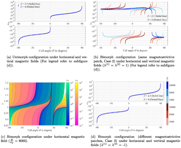
Figure 9. Active modulation of ν21. Variation in ν21 with the change in externally applied magnetic field intensity to σ2 ratio  . The legends for the unimorph and the bimorph configurations are same in all the plots i.e. the legends in subfigure (d) are applicable to the subfigures (a) and (b). The red and blue color in the legend (subfigure (d)) represent the magnetic field intensity to stress ratio in horizontal and vertical directions, respectively. The increase in the color gradient for the red and blue color signifies the increase in the magnetic field intensity to stress ratio. In the contour plot (subfigure (c)), the first and second color bars represent positive and negative Young's modulus, respectively. Different values of β is shown for unimorph (refer to subfigure (a)) and bimorph (refer to subfigures (b) and (d)) configurations. The upper and lower subplots in subfigures (a), (b) and (d) represent the positive and negative values of Poisson's ratio respectively with the change in the cell angle. Sign reversal is clearly visible as the cell angle and the magnetic field to stress ratio is varied. Contour plot (subfigure (c)) shows the variation in ν21 as the cell angle and λ (where,
  = λ) vary at a constant
  ratio.
Download figure:
Standard image High-resolution imageThe variation in the  for unimorph, bimorph (with same magnetostrictive patch) and bimorph (with different magnetostrictive patch) can be observed from figures 6(a), (b) and (d) (refer to case 1, case 2 and case 3 defined in section 3.3). In the unimorph case, when only magnetic field is applied, both axial and transverse displacements can be obtained whereas, in bimorph case 1, the value of transverse displacement and in case 2, the value of axial displacement under applied magnetic field become zero. This variation in the bimorph case can be obtained by keeping different values of λ (where,
  = λ) (here 1 and −1 for the individual cases). Figures 6(a) and (d) show that for unimorph and the bimorph case 2, when the horizontal magnetic field is applied, the sign reversal and variation in
  can be observed. However, in bimorph case 1, sign of
  is positive for the entire range of the cell angle, while the variation with the magnetic field is observed as β and
  vary. On the other hand, under the influence of the vertical magnetic field, the sign reversal and variation are observed for all the three cases for
  . It should be noted that in all the plots, the lines merge at one point when the cell angle is 45∘. This is due to the fact that at this particular cell angle, the value of the vertical and the horizontal component of the applied magnetic field is equal. Hence, there is no effect of the magnetic field on the properties of the lattice structure. The contour plot in figure 6(c) shows the variation in
  as the λ and cell angle varies when the value of
  is kept constant (8000, magnetic field intensity in vertical direction). The value of λ helps in selecting the magnetostrictive patch with specific magnetostrictive coefficient for the top and the bottom surfaces, respectively, so as to obtain the desired set of properties. For a more comprehensive understanding, contour plots for different
  ratios (horizontal and vertical) have been presented in the supplementary material.
For the Poisson's ratio  , in unimorph configuration, there are some instances where the sign reversal can occur as
  ratio is varied, but the range of cell angle is small as shown in figure 7(a). However, the variation in
  occurs as the value of β is varied. For the bimorph case 1, the scenario is completely different as the sign reversal and variation in Poisson's ratio can be observed for the entire range of the cell angle as the
  ratio changes (refer to figure 7(b)). In the bimorph case 2, no significant variation in
  can be observed as shown in figure 7(d). Contour plot shown in figure 7(c) shows the variation in ν12 as the λ and cell angle vary when the value of
  is kept constant (8000, magnetic field intensity in horizontal direction). Figure 7(c) shows that in order to have negative Poisson's ratio when the cell angle is positive, the value of λ has to be less than 1.05. In the supplementary material, additional contour plots for different
  ratios (horizontal and vertical) have been presented.
The variation and sign reversal in the  for unimorph and bimorph configurations can be observed from figures 8(a), (b) and (d) respectively. The variation and sign reversal in
  can be observed in all the cases; however, for the bimorph case 1 under the influence of the vertical magnetic field, no sign reversal for
  has been observed. The contour plot in figure 8(c) shows the variation in
  as the λ and cell angle vary when the value of
  is kept constant (8000, magnetic field intensity in horizontal direction). In the supplementary material, additional contour plots for different
  ratios (horizontal and vertical) have been presented.
For ν21, no variation in unimorph and bimorph case 2 has been observed as the  ratio changes (refer to figures 9(a) and (d)); however, the variation can be observed for different β values. For the bimorph case 1, both sign reversal and variation in Poisson's ratio can be observed under the influence of both vertical and horizontal magnetic fields. The contour plot presented in figure 9(c) shows the variation in ν21 as the λ and cell angle varies when the value of
  is kept constant (8000, magnetic field intensity in horizontal direction). In the supplementary material, additional contour plots for different
  ratios (horizontal and vertical) have been presented.
Figure 10 shows the graphical comparison (bar plot) for the Young's modulus ( and
and  ) and Poisson's ratio (
 and
and  ), considering the bimorph case having same magnetostrictive patches. In each plot, three different sets of six bars represent three different cell angles (30∘, 60∘ and
  ). The different color in the six bars shows the variation in the direction of the externally applied magnetic field to stress ratio, where the red and blue colors stand for horizontal and vertical direction respectively. The change in the magnitude of the externally applied magnetic field to stress ratio is shown by the variation in the gradient of the red and blue color. Figure 10 provides a clear quantitate perspective of the active modulation of elastic properties for different cell angles.

Figure 10. Quantitative comparison of elastic properties. The variation in the elastic properties ( ,
,  ,
,  and
and  ) as the direction and magnitude of the magnetic field intensity to stress ratio is varied. The red and blue color in the legends represent the magnetic field intensity to stress ratio in horizontal and vertical direction, respectively. The increase in the color gradient for the red and blue color signifies the increase in the magnetic field intensity to stress ratio. The values have been plotted for the bimorph case having same magnetostrictive patches (case 2) (
 =
=  = 1) and β = 2.5.
Download figure:
Standard image High-resolution image5. Summary
A computational framework to understand the active modulation of Young's modulus and Poisson's ratio in a contactless manner has been reported in this article. Conditions under which the variation and sign reversal can take place have been discussed through numerical results. The analytical derivation and numerical results provide necessary physical insights and background for potential applications in various futuristic multi-functional structural systems and devices. The major outcomes and observations of the current investigation are summarized below.
- The current framework allows active on-demand modulation of the Elastic properties and Poisson's ratio in a contactless manner. Such controlled variation has been realized by changing the magnetic field intensity to stress ratio .
- The current formulation has been presented in a general form, and all sorts of possible parameters (unimorph, bimorph, identical magnetostrictive patches and dissimilar magnetostrictive patches) can be varied, which provides flexibility in designing active lattice structures as per the requirement of the application.
- Besides achieving an on-demand control over the elastic properties it is possible to have extreme properties like negative effective Young's modulus, or auxetic behavior in structurally non-auxetic lattices and vice-versa.
- The variation and sign reversal in and with the change in magnetic field intensity to stress ratio has been obtained for all the cases. However, in the bimorph case 1, the sign reversal is not observed in two scenarios: under horizontal magnetic field and under vertical magnetic field.
- The variation in and is possible only in the bimorph case 1 under both horizontal and vertical magnetic fields. However, for in unimorph configuration, there exist some instances where sign reversal is possible, but the range is relatively small. Except these, there is no other scenario where the sign reversal or variation in Poisson's ratio is possible.


6. Conclusions and perspective
This article proposes a new class of magnetostrictive hybrid lattice metamaterial constructed using a passive substrate beam and active magnetostrictive patches. A contactless on-demand modulation of effective Young's modulus and Poisson's ratio can be achieved in such materials as a function of an external magnetic field. The hybrid design space in the proposed lattices includes conventional unit cell level microstructural geometry and the intrinsic material properties (passive parameters) along with the intensity and direction of the external magnetic field (active parameters). A bottom-up approach has been followed here to derive efficient analytical expressions of the effective elastic properties considering both axial and bending deformations. The proposed formulation is quite generic as it has been derived to consider different materials for the substrate beam and various configurations of the magnetostrictive patches along with unit cell level geometries. The obtained expressions hold good for unimorph and bimorph (with same and different magnetostrictive patches) configurations along with the horizontal and vertical directions of the magnetic field. A two-step validation approach involving active beam-level deformation physics and unit cell level tessellations has been presented to garner adequate confidence in the developed computational framework.
The mechanical properties of conventional passive lattice materials are predominantly an intrinsic geometric function of the microstructural topology, wherein there is no possibility to alter the properties after manufacturing if the application requirement changes. The incorporation of magnetostrictive patches in the current proposition allows active modulation of elastic properties as per real-time demands. Further, the elastic properties can be controlled in a contactless manner through external magnetic fields, wherein it is not necessary to have any complex non-structural elements (such as circuits) within the metamaterial microstructure. The numerical results reveal that a wide range of active on-demand variations can be achieved in the Young's moduli and Poisson's ratios as a function of the applied magnetic field including extreme cases such as sign reversal (with negative effective Young's modulus and auxetic behavior in structurally non-auxetic lattices or vice-versa). For bimorph lattice structure having cell angle of 30∘, in terms of absolute magnitude active variation of  6 times and
  3 times have been observed in the longitudinal and transverse Young's modulus respectively. For the
  and
and  a variation of about ≈15 times have been observed, which necessarily means that the same material can behave both like a soft polymer or a stiff metal depending on the functional demands. The developed computational framework is directly adaptable to rectangular and rhombic lattices (by considering the cell angle and length of the vertical member as zero, respectively) and it can further be extended to other 2D and 3D lattices by considering appropriate unit cells. The proposed hybrid honeycomb lattice metamaterial can find a wide range of applications, such as actuator, active vibration control, programmed wave guiding by modulating the internal structure of the lattice, controlling energy harvesting, multi-directional stiffness control, energy absorption, soft robotics and shape morphing.
Acknowledgments
The authors acknowledge the financial support from Visvesvaraya PhD scheme, Media Lab Asia, Ministry of Electronics and Information Technology, Government of India, through a scholarship (Unique Awardee No. MEITY-PHD-888) and SPARC Project (MHRD/ME/2018544). T M would like to acknowledge the support received through the Science and Engineering Research Board, India (Grant No. SRG/2020/001398). S A acknowledges the support of the UK-India Education and Research Initiative through Grant No. UKIERI/P1212.
Data availability statement
The data that support the findings of this study are available upon reasonable request from the authors.
Conflict of interest
The authors declare that they have no known competing financial interests or personal relationships that could have appeared to influence the work reported in this paper.
Supplementary data (5.1 MB PDF)