

Abstract
Designing bridges with spans larger than 2000 m is challenging. One critical problem is that the flutter stability of such bridges is extremely weak. In past studies, actively controlled flaps were found to improve the flutter stability performance. However, in those studies, the deck was always assumed to be an ideal streamlined plate to simplify the aerodynamic interference effect in the deck-flap system. This simplification limits the application of this technique on real projects. To improve the applicability, we adopt a typical bluff body deck to investigate the effect of the active flaps under different wind attack angles. The novelty of this work is the analysis of the aerodynamic interference and resulting control impact considering the application scenario. The tests are conducted through the computational fluid dynamic method. To give intuitive explanations of the aerodynamic interference, the distributed aerodynamic characteristics method is innovatively introduced to quantify the contribution of flap on the flutter stability during the control process. Our results show that the leading flap has a dominant contribution to the flutter stability by inducing the beneficial aerodynamic damping on the deck's leading surfaces. Its optimal phase should be about π/2 lagging from the deck's torsional motion. In comparison, the effect of the trailing flap is unstable under different wind attack angles. To guarantee a robust control effect, it is suggested that it remains stationary.
Export citation and abstract BibTeX RIS
1. Introduction
Aerodynamic flutter is a critical wind-induced catastrophic phenomenon for long-span bridges owing to the divergent deck oscillation. Flutter control has attracted much attention since the Tacoma Narrows Bridge disaster. Passive control methods, including shape optimization (Sato et al 2000, Irwin 2008), aerodynamic appendages (Larsen et al 2000, Kitagawa 2004, Yang et al 2017, Starossek et al 2018), and mechanical facilities (Wilde et al 1999, Omenzetter et al 2000, Casalotti et al 2014), have been proved effective when the span is below 2000 m. These techniques can raise the critical flutter-onset wind speed beyond the design wind speed. However, when the span becomes larger, the natural frequency and damping ratio of the bridge decrease significantly, which makes the flutter control more difficult to maintain using a passive control technique (Kubo 2004).
To surpass the limit of the passive controls, some active control solutions were proposed. These solutions focused on the dependencies on the external energy and real-time monitoring. Actively controlled plates have attracted significant attention because their control force can be realized through a comparatively small driving force by taking the advantage of wind force itself. To simplify the mathematical model during deriving the control strategy, the plates were first mounted far away from the bridge deck, as shown in figure 1(a), so that the aerodynamic interference between the deck and the plates could be minimized. This approach is referred to as the 'active winglets' technique. Wilde and Fujino (1998) and Nissen et al (2004) analyzed the control effect of the active winglets through a mathematical model. Kobayashi and Nagaoka (1992) and Liu (2017) realized the physical application of the active winglets in a wind tunnel, which successfully raised the critical flutter speed of a target bluff body deck. Guo (2013) discussed the necessity of the closed-loop control by comparing it with an open-loop control. Li et al (2017) further developed this method and established a general framework to handle arbitrary deck shape and dynamic characteristics. Recent studies took a series of studies of the winglets both in a passive manner and active manner (Phan 2017, Truong and Phan 2021). Sangalli and Braun (2020) compared the control effect between cases with different deck shapes, including rectangular and ellipsoidal, and an actual deck outline, through three-dimensional large eddy simulations. Although the active winglets have shown a strong capacity for flutter control, the winglets must be mounted far from the deck to avoid complex interference effect between winglets and deck. Such a requirement makes this technique difficult to apply in a real project.

Figure 1. Demonstration and comparison between active winglets and active flaps.
Download figure:
Standard image High-resolution imageTo further improve the operability, the active plates were mounted beside the deck's edges (active flaps; shown in figure 1(b)). Hansen and Thoft-Christensen (2001) established a bimodal sectional model with the Theodorsen function, and they successfully realized the flutter suppression of an ideal flat deck in wind tunnel tests. Boberg et al (2015) extracted the flutter parameters of a flat deck and its flaps through wind tunnel tests and pointed out the necessity of considering the interference effect between the bluff body deck and the nearby flaps. Zhao et al (2016) utilized the  hybrid strategy to control the flaps. Additionally, Zhuo et al (2020) proposed a control method depending only on the leeward flap, and the computational fluid dynamics (CFD) simulations showed a good effect with limited energy consumption. Although studies have shown the prominent advantage of active flaps, this technique is limited in the control of ideal plates. This is because, if a bluff deck is involved in the bridge-flap system, it induces more complex aerodynamic interference between the deck and flaps. Such an effect makes it almost impossible to build an analytical expression of the system's aerodynamic forces, according to the potential flow theory.
Regardless of whether the studies investigated active winglets or active flaps, these techniques do not consider the interference effect between the additional plates and deck. This is a serious limitation to these techniques' applicability in real-world scenarios. This study examine the control performance and the control mechanism of a bridge-flap system with an actual bluff body deck through the CFD simulation method. The distributed aerodynamic characteristics technique is innovatively introduced to quantify the aerodynamic interference during the control process. To our knowledge, it is the first time that the aerodynamic interference and the resulting control impact are analyzed by considering the application scenario.
This study is organized as follows. In section 1, the mathematical model of the bridge-flap system is introduced, and the aerodynamic parameters of the ideal-plate case are given as the baseline. Then, in section 2, the CFD method is introduced to obtain the corresponding parameters of the case with an actual bluff deck. In section 3, the impact of the wind attack angle is discussed. In section 4, a phase-shift control algorithm is used. The relationship between the phase value and the control effect is analyzed, and corresponding optimal control laws are discussed. In section 5, based on chosen control laws, the model is made into a classical bimodal flutter model. The interference effect is then analyzed using the method of the distributed aerodynamic characteristics, and the contributions of the flaps are highlighted by demonstrating the sources of the control-induced aerodynamic damping.
2. Mathematical model of the deck-flap system
The mathematical model is based on a sectional bridge-flap system. Figure 2 defines the positive directions of the total wind loads ( represents the force and
  represents the torque) and the degrees of freedom (DoFs, namely,
  ).
).

Figure 2. Forces and DoFs of a sectional deck-flaps model.
Download figure:
Standard image High-resolution imageIn bridge wind engineering, the wind forces acting on the bridge members are usually decomposed into three components: the static component (caused by the long period mean wind speed), the buffeting component (caused by the short period fluctuating wind), and the self-excited component (caused by the fluid-structure interaction). For the active control technique studied here, the static load can be ignored by setting the equilibrium position as the origin of the dynamic equation. The buffeting load is commonly believed to have little influence on the flutter stability and its impact can be considered a challenge to the control robustness (Zhou et al 2019, Hu et al 2021).
When the flap is installed in the same plane as the bridge deck, the aerodynamic interference effect is very strong. The flap's vibration not only affects its own surrounding flow, but also the deck's surrounding flow. This makes the aerodynamic force of the deck-flap system indivisible. Besides, the deck-flap system's force should reflect the influences from all independent DoFs. Referring to Scanlan's flutter theory (Scanlan and Tomko 1971), the motion of the deck-flap system can be decomposed into four parts, namely, the deck's vertical DoF, the deck's torsional DoF, the leading flap's rotational DoF and the tailing flap's rotational DoF. Finally, the forces acting on a unit length deck-flap system can be expressed as
where  and
and  are the total lift force and the total lift moment of the system, respectively.
  is the air density;
  is the circular frequency of the system's sinusoidal oscillation; and
  is the half width of the system. The aerodynamic parameters are denoted by
  and
and  , distinguished by subscripts of the DoFs, which are determined by the shape of the deck and the flaps. They are functions of the reduced frequency
  , in which
  is the mean value of the wind speed. During active control, the dominant frequency of the system's response is determined by the flaps' oscillation, so it should be noted that
  is not the structural modal frequency.
When the deck and the flaps are thin and smooth, and oscillate with a small amplitude under a zero wind attack angle, the aerodynamic parameters' analytical solution can be derived based on the potential flow theory, listed in table 1 ( is an imaginary number). They were cited as the baseline in the following sections, to discuss the influence of the bluff body deck shape and the wind attack angle. The derivation process can be found in a study by Graham et al (2011). For details of
  and
and  , please refer to Theodorsen (1935).
Table 1. Aerodynamic parameters under the ideal-plate assumption.
| Parameter | Value |
|---|---|

|

|

|
|

|
|

|
|

|

|

|
|

|
|

|

|
3. Case setting and validations of the CFD simulations
To investigate the behaviors of an actual bridge-flap system, CFD simulations were introduced to obtain actual aerodynamic parameters, with a typical deck (the Great Belt East Bridge) under a series of wind attack angles. The results are compared with the ideal cases in table 1. The computational domain and the boundary setting are shown in figure 3, with a blockage ratio of 0.95%. An ignorable gap was set between the deck and the flaps, considering the convenience of the mesh generation. To avoid grid distortion near the deck surface during the oscillation process, three computational regions were defined (Miranda et al 2014, Patruno 2015). The rigid zone was used to keep the mesh shape constant, outside which the deforming zone was used to realize the smoothing and remeshing treatments. Then, the outmost fixed zone satisfied the blockage ratio requirement.

Figure 3. Demonstration of the computational domain and the boundary setting.
Download figure:
Standard image High-resolution imageThe simulations were conducted using Ansys Fluent. The Semi-Implicit Method Pressure-Linked Equations Consistent algorithm was used, with second-order scheme for the pressure equation and second-order upwind scheme used for the momentum equation. The unsteady Reynolds-averaged Navier–Stokes equations were used with the  SST turbulence model (Menter 1994) because of their good balance between accuracy and computational cost. The Reynolds number (Re) was
  , with a reference length
  . To prevent the grid from distorting during the object's motion, the range of the diffusion parameter was set between
  and
and  . Increasing this diffusion parameter can make the far-field grids absorb more deformation.
Several validations were conducted to guarantee the correctness of the obtained results in this study. The sensitivity of spatial division and time division to the aerodynamic parameters ( and
and  in equation (1)) was examined. As the aerodynamic parameters are relative to the deck's vibration frequency and the wind's speed, the sensitivity should be tested under different reduced wind speeds (
 ). When determining the to be tested
  , three factors were considered. First, the highest wind speed (
 ) should be lower than the flutter critical wind speed, which is about
  for long-span suspension bridges. Second, the circular frequency (
 ) of the flutter mode is generally 0.6–1.3 (Starossek and Starossek 2021). Third, the half width (
 ) of the bridge is generally 15–17.5 m. Therefore, the sensitivity validation was conducted under
  and
and  , which can almost cover the
  range involved in the control problem. Based on the error-changing tendency of the aerodynamic parameters (table 2), the grid density and the time step were determined considering the balance between accuracies and efficiencies. As the truth data is unknown, the densest grid and the shortest time step was chosen as the reference. When the mesh was adjusted from sparse to dense, the non-dimensional grid height
  at the deck surface changed from 10 to 0.75. Using
  as the baseline, it is noticeable that the relative errors converged rapidly with increasing grid density. When
  , the relative error was stable and small enough. Further reducing the mesh size had a limited effect on improving the calculation accuracy, and resulted in a large calculation consumption. Similar validations were conducted to select a reasonable time step. The maximum courant number was located at the leading surface of the deck, and ranged from 13.6 to 0.68, with reducing time steps. Considering the 0.68 case as the baseline, results showed acceptable precision when the maximum courant number was 1.7. Finally, the spatial division and the time division plans were determined.
Table 2. Sensitivity of the aerodynamic parameters.

| Maximum relative error (%) | Courant number | Maximum relative error (%) | ||
|---|---|---|---|---|---|

|

|

|

| ||
| 0.75 | — | — | 0.68 | — | — |
| 1 | 0.84 | 0.57 | 1.4 | 0.2 | 0.15 |
| 1.25 | 5.21 | 1.74 | 1.7 | 0.23 | 0.19 |
| 2.5 | 5.72 | 2.37 | 3.4 | 0.71 | 0.69 |
| 4 | 4.49 | 3.80 | 6.8 | 5.42 | 2.03 |
| 6 | 7.80 | 3.46 | 13.6 | 15.77 | 4.94 |
To further examine the CFD simulations, mode characters at different wind speeds were calculated using the obtained aerodynamic parameters. The flutter critical velocity was obtained based on a two-DOF model (heaving and pitching). The involved dynamic characteristics of the bridge are listed in table 3. A traditional frequency searching method was used to seek correct heaving and pitching frequencies where frequency-dependent aerodynamic parameters were calculated based on linear interpolation (Xu et al 2022). The calculated flutter critical speed  = 72 m s−1 was close to the observed 73 m s−1 in wind tunnel tests (Larsen 1993, Larsen and Walther 1997), as shown in figure 4. It is noticeable that the overall effect of the simulated self-excited force is satisfactory in accuracy, indicating that the following investigations are expanded based on the foundation of reliable data.

Figure 4. Dynamic characteristics of the heaving and pitching modes at different wind speeds.
Download figure:
Standard image High-resolution imageTable 3. Dynamic characteristics of the great belt bridge.
| Dynamic characteristics | Denotation | Unit | Value |
|---|---|---|---|
| The equivalent mass |

|

| 22.70 |
| The equivalent mass moment of the inertia |

|

| 2470 |
| The circular frequency of the heaving mode |

|

| 0.628 |
| The damping ratio of the heaving mode |

| — | 0.2% |
| The circular frequency of the pitching mode |

|

| 1.747 |
| The damping ratio of the pitching mode |

| — | 0.2% |
To obtain the necessary data for the following involved issues, sinusoidal forced vibrations under different wind attack angles, reduced wind speeds ( ), and vibrating DoFs (
 ) were investigated (a total of 220 cases), and the data are shown in table 4. The amplitude of the torsional vibration was 2°, and the amplitude of the vertical vibration was equal to the deck's edge displacement during the torsional vibration. The aerodynamic forces (
 ) and the pressure distributions on the deck surface were recorded at a constant time interval in each case.
Table 4. Case setting of the forced vibrations.
| Case differences | AoA | DoFs |

|
|---|---|---|---|
| Range |
 to to 
| Rigid body motion: vertical and torsional local deformation: leading flaps and trailing flap |

|
| Interval |

| — | 2 |
4. Interference's impact on the motion induced force
According to equation (1), the force acted on the deck-flaps system is the superposition of four parts. Among them,  ,
,  ,
,  , and
, and  represent the contributions from the rigid-body motions, indicating the flaps are stationary relative to the deck. Based on these four parameters, the interference's impact on the rigid-body motion induced force is demonstrated in figure 4. Each subfigure corresponds to different wind attack angles. The dotted lines represent the baseline case following the ideal-plate hypothesis (table 1). When the reduced wind speed increases from 6 to 26, the data move from the circular mark to the hexagonal star mark. The warm color lines represent the contribution to the lift force and the cold color lines represent the contribution to the lift moment. In equation (1), the aerodynamic parameters are expressed as complex numbers. Their real parts represent the proportional factor to the displacement component of the corresponding DoF, while their imaginary parts represent the proportional factor to the velocity component. Therefore, in figure 5, the vector length, pointing from the origin of the coordinates to data points, represents the total aerodynamic force of the corresponding DoF. The angle between the vector and the axes indicates the phase between the aerodynamic force and the vibration of corresponding DoF.

Figure 5. Interference's impact on the rigid-body motion induced force.
Download figure:
Standard image High-resolution imageIn figure 5, it is noticeable that the four aerodynamic parameters' changing tendency showed completely different patterns from those obtained from the ideal-plate case, decided by the wind attack angle's sign. When the wind attack angle was negative, the aerodynamic parameters were similar to the ones in the ideal-plate case. The relatively more obvious change was  : a lower wind attack angle resulted in a shift of the
  line, indicating that the phase difference between the lift force and the rigid-body pithing oscillation is reduced. As for negative wind attack angles, the change of the aerodynamic parameters was very conspicuous compared to the baseline case. When the reduced wind speed was small, the aerodynamic parameters were close to the values of the benchmark. However, with the increase of the reduced wind speed, all of the parameters tended to have the opposite sign of the imaginary parts. Considering the physical meaning of equation (1), the real part of the aerodynamic parameters denotes the force component which is proportional to the displacement, and the imaginary part denotes the force component which is proportional to the velocity. So, the changed proportion of the parameters' real part and the imaginary part indicates that the sign of the phase angle would change when the reduced wind speed was high enough.
Except for the rigid-body motion, the local deformation of the two flaps also provides motion-excited force to the whole system. According to equation (1),  ,
,  ,
,  , and
, and  represent the relationship between the local deformation and the control force. When the flaps' relative angles (
 and
and  ) are manipulated during active control, these components become the control forces suppressing the system's response (
 and
and  ). The interference's impact on these four parameters is demonstrated in figure 6. The configurations of the figures and the case range were identical to those found in figure 5.

Figure 6. Interference's impact on the local deformation induced force.
Download figure:
Standard image High-resolution imageFigure 6 reflects two frustrating aspects. First, the control force provided by the actual flaps was generally far less than the expected level shown in the ideal-plate case. Second, the changed proportion of the real part and imaginary part indicates that the phase relationship between the flaps' motion and their generated force was unstable when the wind attack angle changed. For the force magnitude, the trailing flap only provided 10%–20% of the lift force and 15%–40% of the lift moment, compared to the ideal-plate case. This occurred because the trailing flap was merged in the wake region of the bluff body deck, which is a highly turbulent region, and the deformation of the trailing flap could not significantly affect the flow pattern as that of the lead flap. This result means that the active flap mounted on the trailing edge of real bridge would not be effective as that mounted on the ideal plate. However, the leading flap provided a much larger control force than expected, almost two or three times the value of the baseline case. This result might be caused by the wind acceleration effect of the deck's windward fairing. However, the enhanced control ability of the leading flap could not fully compensate for the reduced value of the trailing flap. The situation becomes more complex in regard to the phase relationship: All four of the parameters show significant (or even opposite) variety when the wind attack angle changed from negative to positive. This change means identical control patterns may result in different control effects. A simple algorithm that can provide a good control effect under all wind attack angles may not exist.
In summary, although the bluff body deck has some severe challenges to the active flap method, the difficulty of the problem is still controllable. First, the parameters' change under different reduced wind speeds is not a problem. Once the target bridge is determined, the structural dynamic characteristics are fixed. Since the flaps' control force is small at a low wind speed, the active control will not affect the system's flutter stability at a low wind speed. It is worthy to note that the optimal control parameters need to be re-calculated if the bridge's dynamic characteristics change. Second, the attenuation of the overall control force is not a significant problem, because the driving force of the flaps (just to change the angle of the flaps) can provide more than ten times the control force for the deck (Li et al 2017). Although the flaps with the bluff body deck need to vibrate more violently than the flaps with an ideal-plate deck, its energy consumption is still much smaller than other active control methods (e.g. active mass damper). Finally, the most challenging problem is the violent change of the phase angle between the aerodynamic force and the vibration of the corresponding DoF under different wind attack angles because the actual wind attacking angle changes all the time. For a typhoon, it usually takes hours for the attacking angle to change its sign, and for a downburst, the time is about several minutes.
5. Relationship between the flaps' motion phase and the control effect
In this section, the sensitivity of the control effect to the flaps' motion phase is analyzed, and the corresponding optimal control patterns are given at different wind attack angles. The feasibility and robustness of active flaps with bluff body deck are discussed.
Near the flutter onset speed, the modes not involved in flutter have large aerodynamic damping, and decay rapidly during the control process. Under such circumstances, the bridge basically presents a single frequency motion. When the feedback control method is applied on the flaps, their vibrations are determined by the deck's motion, and their vibration frequencies are the single frequency that is identical to that of the deck. In a previous study (Guo 2013), it was observed that a steady state existed during the feedback control, in which the phase differences between the flaps and the deck were constant values. This steady state was independent of the initial condition of the control system and control algorithm. The key variables during the steady state were the phase difference between the flaps and the deck, independent of any specified control algorithm. Based on this fact, a simple control algorithm to examine the control phase's impact on the control effect was developed:
where all the binary subscripts indicate the involved two DoFs.  is the gain amplitude and
  is the phase angle. According to equation (2), the flap's motions are decided by the deck's heaving oscillation and pitching oscillation, respectively. Through this method,
  and
and  can be eliminated in equation (1), and the model degenerates into a classical bimodal system, shown as equation (3). The aerodynamic parameters are determined by the combination of the inherent aerodynamic characteristics and the imposed control law, given in table 5.
Table 5. Parameters of the degenerated model under control.
| Parameter | Value ( is an imaginary number) is an imaginary number) |
|---|---|

|

|

|

|

|

|

|

|
Then, an eigenvalue analysis was conducted on equation (3) under different phase settings, ranging from  to
to  , with identical amplification gains. The impact on the control effect is demonstrated in figure 7 by giving the control-induced damping of the flutter mode. The involved color setting was similar to that in figures 5 and 6, and the meaning is given in the figures. Since the magnitude of the control effect can be adjusted by the amplitude of the gain, it is not necessary to compare the control effect between different wind angles. Only the distribution pattern of the control phase matters. Therefore, it is not necessary to set the vertical coordinate axes as the same, and the mean values of the curves have been removed to highlight the change tendency.
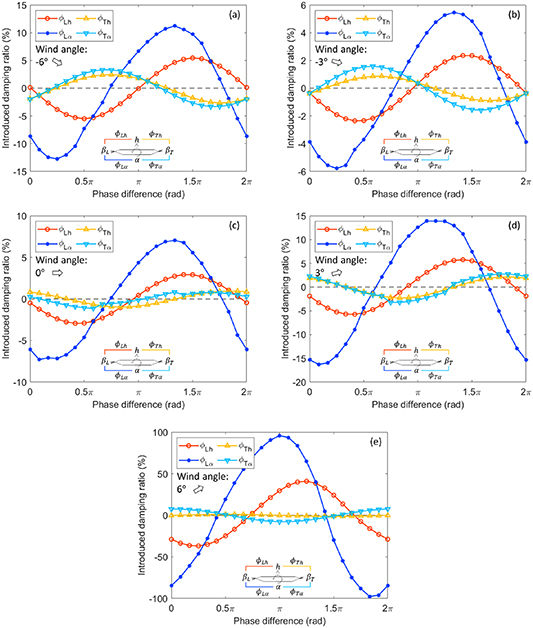
Figure 7. Relationship between the control effect and the control phase.
Download figure:
Standard image High-resolution imageWhen identical gain amplitudes were used on the flaps, the leading flap always had the largest contribution in all wind attack angles. The most important point was that the relationship between the leading flap's phase and the control effect was relatively stable. It indicated a robust control effect to the change of the wind environment. For the optimal control phase, a slight difference was observed under different wind attack angles. For negative wind attack angles, the optimal control occurred during an almost identical situation: when the leading flap's phase was about 1.5 in advance to the deck's vertical oscillation and 1.3
 in advance to the deck's torsional oscillation. For positive wind attack angles, the optimal control phase moved to smaller values, and the change amount ranged from
  to
to  .
.
The control efficiency of the trailing flap was much lower than the leading one. When its gain amplitude was set as identical to the leading flap, the trailing flap only accounted for  %–20% of the total contribution. The robustness of the trailing flap's control ability was poor, because its beneficial control phase changes a lot under different wind attack angles. From the view of optimal control phase, this phenomenon was obvious. The optimal control phase was about 0.7
 for negative wind attack angles, and changed toward zero when the wind attack angle became positive. In actual wind environment, the variation of wind angle of attack is a common phenomenon. If the wind attack angle changed, an originally beneficial control phase could result in a bad effect.
In summary, the control behavior of an actual bridge-flap system is different from that in an ideal plate case. The bluff-body effect greatly increased the challenge of applying this active control system in practice. There are two main aspects worth noting. First, the control efficiencies of the flaps are reversed. The trailing flap's contribution to the flutter stability is far less than what is shown in the ideal-plate case, which may have resulted from the occlusion effect of the deck. Second, the control robustness still satisfies if a dedicated control strategy is applied on the flap pair. One solution is to identify the wind direction so the leading flap can be specified. It can be realized by hardware support, e.g. using anemometers. Another solution is to introduce a complex algorithm, e.g. utilizing the vibration center offset phenomenon in modal coupling to discriminate between the flaps or introducing a nonlinear self-adapting control law through reinforcement learning techniques.
6. Distribution of the control induced aerodynamic damping
In previous sections, the control strategy of the flaps was discussed but the improvement of the flutter stability was not given. This is because the degree of the improvement can be adjusted by changing the amplification gain ( ). In other words, once the phases of the flaps are determined, double the leading flap's vibrating amplitude can achieve double damping (under the framework of the linear aerodynamic model used in this paper). In practical operations, the amplification gain cannot be too large, making sure the flap's amplitude not exceeding the stall angle. Besides, the increased flutter speed will not exceed the static divergent speed, even under the best control strategy.
Although the improvement amount of the flutter stability is changeable, the control mechanism is the same when identical control phases are applied. In previous sections, the impact of the aerodynamic interference was discussed through the overall behavior of the bridge-flap system. To give a more intuitive understanding about how the flap influences the system's flutter stability, the distributed aerodynamic characteristics method (Li et al 2019) was introduced. To use this method, the necessary information is the surface flutter derivatives of two DoFs. Therefore, the bridge-flap system, which was originally with four DoFs, needed to be degenerated into a bimodal one.
The distribution of the control induced damping can be calculated refer to equations (15)–(18), proposed by Li et al (2019). Before using these equations, two steps of preprocessing should be introduced. First, the distributed parameters of the deck-flap system should be obtained, defined as equation (4). Since controlling the trailing flap is disadvantageous, only the terms representing the leading flap are kept. Based on the motion induced force acting on the jth piece of the surface (including the deck and the flaps), the surface flutter derivatives are denoted as  ,
,  ,
,  and
and  ,
,  ,
,  . Second, the corresponding parameters should be replaced by those from table 6, where
  and
and  are the real part and imaginary part, respectively. So, the DoF of the leading flap is eliminated, and the remaining DoFs no longer just represent the deck's motion, but represent the control pattern of the deck-flap system.
Table 6. Surface flutter derivatives of the bridge-flap system.
| Parameters in Li et al (2019) | Value |
|---|---|

|

|

|

|

|

|

|

|

|

|

|

|

|

|

|

|
When demonstrating the sources of the control effect, the optimal control phases under each wind attacking angle were decided based on figure 7, and the results are listed in table 7. The distributions of the control-induced aerodynamic damping are demonstrated in figure 8. The positive (beneficial) damping corresponds to the direction pointing outward from the deck's surface.

Figure 8. Distribution of the control-induced aerodynamic damping.
Download figure:
Standard image High-resolution imageTable 7. Control phases used to demonstrate the control mechanism.
| Parameter | Wind attack angle | ||||
|---|---|---|---|---|---|

|

|

|

|

| |

| 4.712 | 4.451 | 4.451 | 4.451 | 3.927 |

| 4.189 | 4.189 | 4.189 | 3.665 | 3.142 |
The results reflected a unique control mechanism. The control effect came from not only the flap, but the deck itself. Such a mechanism was much different than one that was involved in the active winglets case (figure 1). When the flaps and the deck were adjacent, they shared a common boundary layer. The flap's vibration stirred the surrounding flow, showing a strong interference phenomenon. From the view of flutter control, the aerodynamic damping not only came from the flap itself, but also from the deck. The deck zone behind the leading flap always provided a positive damping, regardless of the change of the wind attack angles. Its magnitude was of the same order as the damping contributed by the flap. The benefiting surface was always located at the downstream zone of the flap, namely, at the upper surface when the wind attack angle was negative and at the lower surface when the wind attack angle was positive. When the wind attack angle ranged from  to
to  , the leeward part of the deck and the stationary flap both had little effect on the flutter control. This conclusion was altered when a large positive wind attack angle occurred. All of the leeward surfaces contributed a significant positive damping effect, which offset a large amount of the enhanced negative damping from the windward part of the deck.
In section 5, the optimal control phase of the leading flap was given. It almost maintains identical when the wind attack angle changes. So, in a simplified control law, the phase of the leading flap can be about π/2 lagging from the deck's torsional motion, which is demonstrated in figure 9. This figure shows that the leading flap should have the maximum angular velocity when the deck reaches the torsional amplitude. It should have the maximum angular displacement when the deck passes through the equilibrium position. Besides, the trailing flap should remain stationary to guarantee a robust control effect, in case of a sudden change of the wind attack angle.

Figure 9. Demonstration of the optimal control pattern.
Download figure:
Standard image High-resolution image
7. Conclusion
We investigated the actual behavior of the active-flap method using a typical bluff deck instead of the commonly assumed ideal-plate deck, and varying wind attack angles (from  to
to  ) were involved. First, the control effectiveness was examined by analyzing the force components of the bridge-flap system. Second, the control robustness was examined by comparisons between different control phases. Finally, the control mechanism was revealed by demonstrating the sources of the control force through the distributed aerodynamic characteristics. The leading flap dominated the flutter stability during the active control. It provided a robust and large control force under all wind attack angles. Its optimal phase was about π/2 lagging from the deck's torsional motion, and it can stimulate the deck's nearby surfaces to generate beneficial aerodynamic damping. The trailing flap showed a changing control effect with varying wind attack angles, which was fatal to the control robustness. It should remain stationary during the control process.
Acknowledgments
This work was supported by the National Science Foundation for Young Scientists of China (51808075), the National Natural Science Foundation of China (52078087), 111 Project (B18062), the Natural Science Foundation of Chongqing, China (cstc2020jcyj-msxmX0773), and the Fundamental Research Funds for the Central Universities (2020CDJ-LHZZ-018). We thank LetPub (www.letpub.com) for its linguistic assistance during the preparation of this manuscript.
Data availability statement
The data that support the findings of this study are available upon reasonable request from the authors.