

Abstract
Due to the complex nonlinearity of magnetorheological (MR) behavior, the modeling of MR dampers is a challenge. A simple and effective model of MR damper remains a work in progress. A novel model of MR damper is proposed with force-velocity hysteresis division method in this study. A typical hysteresis loop of MR damper can be simply divided into two novel curves with the division idea. One is the backbone curve and the other is the branch curve. The exponential-family functions which capturing the characteristics of the two curves can simplify the model and improve the identification efficiency. To illustrate and validate the novel phenomenological model with hysteresis division idea, a dual-end MR damper is designed and tested. Based on the experimental data, the characteristics of the novel curves are investigated. To simplify the parameters identification and obtain the reversibility, the maximum force part, the non-dimensional backbone part and the non-dimensional branch part are derived from the two curves. The maximum force part and the non-dimensional part are in multiplication type add-rule. The maximum force part is dependent on the current and maximum velocity. The non-dominated sorting genetic algorithm II (NSGA II) based on the design of experiments (DOE) is employed to identify the parameters of the normalized shape functions. Comparative analysis is conducted based on the identification results. The analysis shows that the novel model with few identification parameters has higher accuracy and better predictive ability.
Export citation and abstract BibTeX RIS
1. Introduction
As a kind of smart actuator, magnetorheological (MR) dampers possess many salient characteristics such as rapid response, controllability, reversibility and low power requirement. The MR dampers working at shear mode, valve mode, squeeze mode or their mixed modes have been primarily and successfully applied in some engineering situations (e.g., vehicle suspension [1, 2], seat [3], bridge [4–6] and building [7, 8] and so on [9]). However, the MR damper provides the excellent characteristics on the one hand, the complex nonlinear hysteresis behavior of MR damper causes the challenge in control applications on the other hand. A dynamic model of MR damper with high accuracy is necessary. It is noted that the dampers working in different modes display different nonlinear hysteresis behavior characteristics, for example, the force-velocity and force-displacement loops of the MR actuator working in shear mode, valve mode and their mixed mode are rate-dependent while the characteristics of the MR actuator working in squeeze mode is rate-independent [10]. Until now, the dynamic models are mostly constructed for the MR damper working at shear mode, valve mode and their mixed mode. These dynamic models can be classified into the mechanism models and the phenomenological models. The mechanism models are derived from the working mechanism of the MR damper. The parameters in the mechanism models have specifically physical meanings such as the spring, the viscous dashpot, the coulomb friction element, the mass, etc. The typical mechanism models include the Bingham plastic model [11], the modified Bingham model [12, 13], the lumped parameter model [14, 15], the visco-elastic-plastic model [16], the equivalent model [17] and so on. The simple Bingham plastic model cannot portray the hysteretic properties under lower velocities. Therefore, different elements were introduced to improve the accuracy of the model. The modified Bingham models introduced the spring element to present the series compliance in the damper. The fluid inertia was proposed in the lumped parameter model. The visco-elastic-plastic model considered the effects of the fluid viscous residence and fluid inertia component in post-yield region. The additional stiffness element was introduced in the equivalent model to describe the MR fluid's compressibility. Different from the mechanism models, not all the elements in the phenomenological models have the physical meanings. The phenomenological models rely largely on the shape functions to describe the non-linear hysteretic characteristics. The existing shape functions contain the differential equations [18–20], trigonometric-family functions [21, 22], exponential-family functions [23, 24], piecewise functions [1, 25, 26] and so on [27–30].
The phenomenological models with different shape functions have their specific properties. The representative of the models with differential equations is the Bouc-Wen model. To capture the force-displacement and force-velocity behaviors accurately, several improved versions of the Bouc-Wen models and Dahl modes [4, 5] have been studied. These models with the differential equations are complicated and difficult to solve. In addition, the identification process is time-consuming because of the frequently occurred divergence problem [31]. There are several algebraic dynamic models constructed from the trigonometric-family functions. Kwok et al [22] proposed a model with the hyperbolic tangent function to represent the hysteretic characteristics. This model can be computationally efficient due to the few identification parameters. Guo et al [21] and Sahin et al [31] proposed the models using the arctangent functions. In Sahin's study, these algebraic models are more simple and efficient than the models with differential equations. The elements in the models with the differential equations and trigonometric-family functions are all combined in addition-type add-rule which cannot be resolved to obtain the current easily [32, 33]. In addition, the exponential-family functions containing the sigmoid function and Gauss function are utilized widely in the hysteretic models, for example, the enhanced Bouc–Wen model [34], the sigmoid models [23, 24], the neural networks models [35] and the adaptive-network-based fuzzy inference system (ANFIS) models [36]. To improve the conventional Bouc–Wen model to describe the response of a rotational MR damper, an enhanced Bouc–Wen model coupled with a sigmoid function is proposed in the study of Miah et al [34]. The sigmoid model is composed of the velocity-dependent part and current-dependent part in multiplication type add-rule [23, 24]. The models in multiplication type add-rule have superiorities over the models in addition-type add-rule to obtain the control current. With the addition of the computational efficiency of sigmoid functions, the sigmoid model possesses the reversibility. The accuracy of the neural networks model [35] with the sigmoid function and the ANFIS model [36] with the Gauss function are validated. Different from the sigmoid model, force-predicting ability and current-predicting ability of the the neural networks model and the ANFIS model cannot be obtained via one identification process.
The shape functions in the above phenomenological models are used to capture the characteristics of the whole hysteresis loop. To reduce the complexity of finding proper functions for the hysteresis loop, the models with piecewise functions are proposed and analyzed. The hysteresis loop is separated into several regions with the division method. The piecewise functions are utilized to capture the features of different regions in the model. The hysteresis loop was separated into two non-linear curves with sign of acceleration by Choi et al [25]. In the model, two polynomial functions were used to capture the characteristics of the two curves. The polynomial function relying on a large number of parameters to capture the relationships among the force, velocity and current is complex to identify. The force-velocity loop is separated into six regions in the non-linear hysteretic bi-viscous model proposed by Wereley et al [26]. The decelerating yield velocity, accelerating yield velocity and peak velocities are used to connect the regions. An obvious flaw is that the relationship between the identified parameter and current cannot be described by the simple function.
The accuracy describing the difference between the output of the model and the experimental results is the prior condition of modeling. In addition, the reversibility and simplicity are also necessary. The invertible models are still immature and need to be developed due to more studies focus on improving the accuracy of positive dynamic models.
In this study, a novel phenomenological model is proposed to capture the intrinsic nonlinear hysteretic characteristics with the division method. The main contents of this study are as follows. Section 2 shows the force-velocity loop hysteresis division method. Modeling of dual end MR damper via hysteresis division method is analyzed in section 3. The experimental analysis and the model construction are done in this section. The parameter identification and validation are discussed in section 4. Finally, the conclusions are conducted in section 5.
2. Hysteresis division method
To capture the hysteresis properties of MR damper, a novel division method is proposed and analyzed [37]. Figure 1 shows the details of the novel hysteresis division method. As shown in figure 1(a), the ideal hysteretic loop can be divided into two parts with sign of acceleration. The two independent parts are negative acceleration part (upper curve) and positive acceleration part (lower curve), respectively. In figure 1(a),  and
and  are the displacement and acceleration, respectively.
  is the damping force. The mathematical expression of figure 1(a) can be seen in equation (1). In this equation,
  and
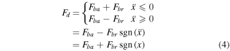
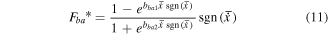
and  are the upper force and lower force, respectively. The upper curve and lower curve are shown in green and blue, respectively. Two new curves can be obtained via operating the upper curve and lower curve which can be seen in equations (2) and (3).
  and
and  are the backbone force and the branch force, respectively. The shape of the new curves can be seen in figures 1(d) and (e).
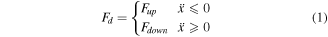


Figure 1. Details of the novel hysteresis division method.
Download figure:
Standard image High-resolution imageTherefore, the force-velocity loop can be divided into backbone curve and branch curve by the novel division method. The mathematical description of the model based on the novel division method is expressed as equation (4).
From figures 1(d) and (e), the backbone curve passing through the zero-force point is center symmetrical curve while the branch curve is symmetrical along the zero velocity line. From figure 1, the new two curves are in the shape of the S-shape curve and Gauss curve, respectively. The exponential-family functions are derived to describe the curves are shown in equations (5) and (6). The force-velocity loops under different frequencies, displacements and current can be captured by changing the parameters' values of a, b, c, d, e and f.

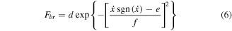
here,  is the damper's velocity. a, b, c, d, e and f are the parameters which are associated with the excitations.
In order to better understand the shape of curves described by equations (5) and (6), the analysis of parametric sensitivity is conducted. The basic reference values of six parameters are 0.5435, −3.2445, −6.7928, 0.2882, 0.05 and −0.314 194 194, respectively. The amplitude and frequency of the excitation are 10 mm and 0.6 Hz, respectively. The curves in figure 2 are obtained based on the parameters' values which calculated via multiplying the reference values by ratio. The values of ratio are −1, −0.5, 0.5, 1 and 5, respectively. With the increment of absolute value of a, the maximum values of curves increase which can be seen in figure 2(a). Comparing the lines, the curves are symmetrical along the zero force line when change the sign of a. From figure 2(b), the curves are in the first and third quadrants when b is negative while the curves are in the second and fourth quadrants when b is positive. The growth rate of the curves in first and third quadrants increase firstly and decrease later. The maximum values of these curves will tend to coincide. The descent rate of the curves in second and fourth quadrants decrease firstly and increase later. From figure 2(c), the absolute values of the curves increase with the decrement of c. When c is positive, the values of curves at the maximum velocities tend to zero. The maximum values of curves increase with the increment of absolute value of d which are shown in figure 2(d). The curves are symmetrical along the zero force line when change the sign of d. The value of e is the symmetry axis of the Gauss curve. The curves will shift with the changing of e which can be seen in figure 2(e). The width of the curve increase with the increment of absolute value of f which can be seen in figure 2(f). The curves coincide when change the sign of f.
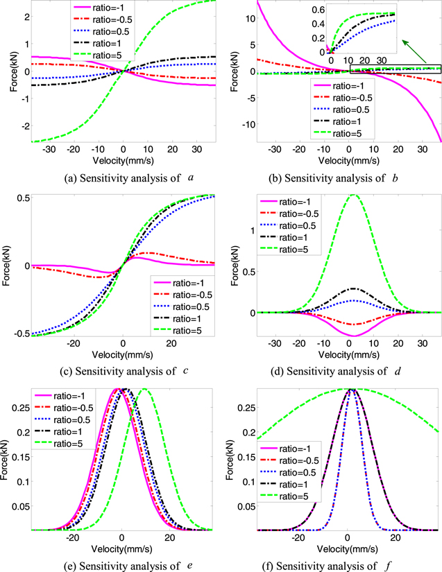
Figure 2. Parametric sensitivity analysis.
Download figure:
Standard image High-resolution image3. Modeling of MR damper via hysteresis division method
3.1. Experimental test of MR damper
To illustrate and validate the novel phenomenological model, the MR damper should be designed and tested. Considering the gas chamber which may affect the saturation of force-displacement and force-velocity loops has been removed from the dual-end MR damper, this type damper is selected here. The 3D diagram of the dual-end MR damper which works at mixed mode composed of shear mode and valve mode is displayed in figure 3. It consists of two piston rods, cylinder, piston, coil and guiding. The structural dimension of the dual-end MR damper is given in table 1. The experimental set-up shown in figure 4 is adopted to evaluate the performance and obtain the force-velocity hysteresis characteristics of the dual end MR damper. The input excitations contain the sinusoidal excitations and current can be seen in table 2.

Figure 3. 3D schematic of the MR damper.
Download figure:
Standard image High-resolution imageTable 1. Dimension of dual-end MR damper.
| Parameters | Dimensions (m) |
|---|---|
| Inner diameter of cylinder | 0.044 |
| Thickness of cylinder | 0.003 |
| Diameter of piston | 0.042 |
| Length of active region | 0.020 |
| Width of coil region | 0.0072 |
| Length of coil region | 0.035 |

Figure 4. Test rig for the MR damper.
Download figure:
Standard image High-resolution imageTable 2. Details of input excitations.
| Excitations | Values | ||||||||
|---|---|---|---|---|---|---|---|---|---|
| Current (A) | 0, 0.2,0.4,0.6,0.8 | ||||||||
| Amplitude (mm) | 5 | 5 | 5 | 10 | 10 | 10 | 15 | 15 | 15 |
| Frequency (Hz) | 0.6 | 0.8 | 1 | 0.6 | 0.8 | 1 | 0.6 | 0.8 | 1 |
| Maximum velocity (mm s−1) | 18.8 | 25.1 | 31.4 | 37.7 | 50.3 | 62.8 | 56.5 | 75.4 | 94.2 |
The experimental results can be seen in figures 5–7. From the figures 5 and 6, the maximum damping force increases with the increment of frequency and amplitude. The maximum damping force increases with the increment of current as shown in figure 7. The force-velocity hysteresis loops appeared along the counterclockwise direction as shown in figures 5(a), 6(a) and 7(a). The upper curves represent the damping force changes with the decreasing velocities while the lower curves show the force changes with the increasing velocities. The strong bi-nonlinear hysteretic characteristic displayed in the pre-yield segment is a typical viscoelastic behavior while the post-yield segment shows plastic characteristics. From figure 7(a), it can be seen that the slope at the post-yield segment increases with the increment of current due to the increased apparent viscosity of MR fluid [38]. Due to manufacturing tolerance, the curves are not so smooth.

Figure 5. Experimental results at amplitude of 15 mm and current of 0.6 A.
Download figure:
Standard image High-resolution image
Figure 6. Experimental results at frequency of 0.8 Hz and current of 0.6 A.
Download figure:
Standard image High-resolution image
Figure 7. Experimental results under different current at amplitude of 15 mm and frequency of 0.6 Hz.
Download figure:
Standard image High-resolution imageFigure 8 shows that the dynamic range decreases with the increment of maximum velocity. The maximum value of the dynamic range in this figure appeared at velocity of 18.8 mm s−1 and current of 0.8 A is 3.32.

Figure 8. Dynamic range vs. maximum velocity.
Download figure:
Standard image High-resolution image3.2. Characteristics of the backbone curves and branch curves
The backbone curves and branch curves under different excitations are shown in figures 9–11. From figure 9(a), the maximum force of the backbone curve increases with the increment of frequency. As shown in figure 9(b), the maximum force of the branch curve and the width of the branch curve increase with the increment of frequency. From figure 10(a), the maximum force of the backbone curve increases with the increment of amplitude. As displayed in figure 10(b), the maximum force of the branch curve and the width of the branch curve increase with the increment of frequency. In figure 11(a), the maximum force of the backbone curve increases nonlinearly with the increment of the current. From figure 11(b), the maximum force of branch curve increase with the increment of current.

Figure 9. Characteristics of two parts at the amplitude of 15 mm and current of 0.6 A.
Download figure:
Standard image High-resolution image
Figure 10. Characteristics of two parts at the frequency of 0.8 Hz and current of 0.6 A.
Download figure:
Standard image High-resolution image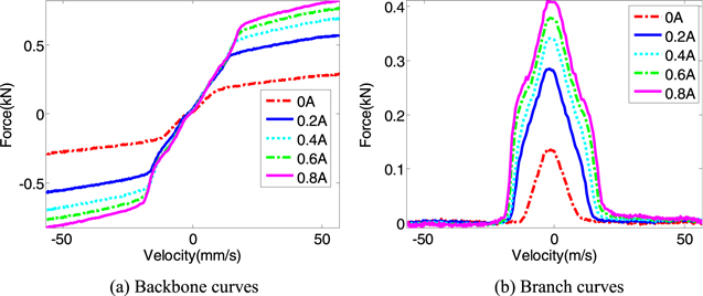
Figure 11. Characteristics of two parts at the amplitude of 15 mm and frequency of 0.6 Hz.
Download figure:
Standard image High-resolution image3.3. Description of the functions
To realize the model based on the experimental results, the normalized method is used here. As one of the data processing methods, normalization method is used to adjust different scale parameters to a common scale by linear transformation. Based on equation (4) and the normalized method, equation (7) is given by

here,  and
and  are the maximum force and the normalized damping force, respectively. The normalized force
  is obtained from dividing the damping force
  to the maximum damping force
  by the normalization method. The maximum and minimum values of the normalized force
  are become to 1 and −1, respectively. The normalized force
  is divided into non-dimensional backbone force
  and non-dimensional branch force
  The relationship between the backbone force and non-dimensional backbone force is
  Similarly, the relationship between the branch force and non-dimensional branch force is
  The maximum force part, the non-dimensional backbone part and the non-dimensional branch part are derived from the two curves. The maximum force part and non-dimensional parts are in multiplication type add-rule which can simplify the parameters identification and obtain the reversibility.
The maximum force part is dependent on the current and maximum velocity. From the current of 0 A to 0.8 A, the non-linear trend between the maximum damping force  and the maximum velocity
  is displayed in figure 12(a). The significant non-linear relationships between the maximum damping force
  and current
  under different maximum velocities are shown in figure 12(b). Combing the principle of the representative quasi-static model- Bingham model, the maximum force
  can be obtained by the maximum velocity-dependent part
  and the current-dependent part
  as shown in equation (8). The
  and
and  described by exponential equations are displayed in equations (9) and (10).


Figure 12. Maximum force characteristics.
Download figure:
Standard image High-resolution imageReferring to the equations (5) and (6), the equations describe the non-dimensional curves are as follows.

here, 


 and
and  are identified parameters. The normalized displacement
  and the normalized velocity
  are obtained as equations (13) and (14), respectively. Their maximum and minimum values are 1 and −1, respectively.


here,  and
and  are displacement and velocity.
  and
and  are maximum displacement and maximum velocity, respectively. The mathematical expression of the maximum velocity is

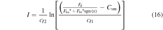
Based on the analysis above, the numbers of the novel model and the number of the shape part are 10 and 5, respectively. The multiplication type add-rule can be ensure the model have the reversibility. The reversibility of the novel model can be obtained as shown in equation (16).
here,  and
and 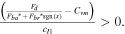 If
If 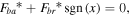 the value of
  would be set as zero.
4. Parameter identification and validation
4.1. Parameters identification
To verify the accuracy of the novel model, parameters identification should be conducted. Before operating the parameters identification, the performance's indices including the mean deviation (MD) and root-mean-square error (RMSE) [39] are defined as
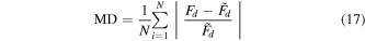
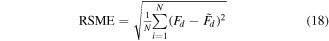
here,  and
and  are identification results and experimental results, respectively. In traditional multi-objective optimization processes, the scalar methods are used as the optimization algorithms. For example, the weighting method which transforms the multi-objectives problem to the single objective problem is one of the typical scalar methods [40]. Unlike the scalar method, the non-scalar method uses the Pareto mechanism to solve the multi-objectives problems. The non-dominated sorting genetic algorithm II (NSGA II) is one of the representational non-scalar methods [41]. To accelerate the convergence of NSGA II, a NSGA II integrated with the DOE method is proposed [42]. The DOE method is used to find the effective design area which can improve the efficiency of the optimal process. Figure 13 shows the schematic of the identification process.

Figure 13. Schematic of the identification process.
Download figure:
Standard image High-resolution imageThe values of the identified parameters are shown in table 3. Comparison between the experimental results and the identification results can be seen in figures 14–16. From these figures, it can be seen that the novel model can fit the experimental data well. The hysteresis characteristics, controllability, the flux saturation and frequency dependence are all validated.
Table 3. Values of identified parameters.
| Parameters |

|

|

|

|

|
|---|---|---|---|---|---|
| Values | −3.2445 | −6.7928 | 0.004 562 | 0.530 36 | −0.314 194 194 |
| Parameters |

|

|

|

|

|
| Values | 0.283 942 857 | 0.705 676 127 | −0.028 08 | −0.5568 | −3.724 |

Figure 14. Comparison between the experimental results and identification results at amplitude of 5 mm.
Download figure:
Standard image High-resolution image
Figure 15. Comparison between the experimental results and identification results at amplitude of 10 mm.
Download figure:
Standard image High-resolution image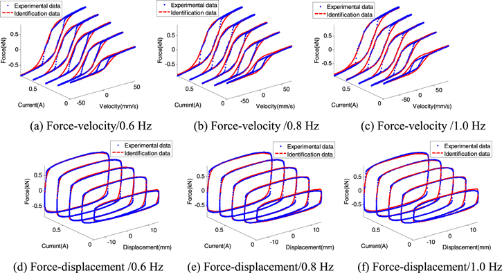
Figure 16. Comparison between the experimental results and identification results at amplitude of 15 mm (blue dot—experimental results; red dashed line—identification results).
Download figure:
Standard image High-resolution imageThe values of MD and RMSE under different excitations are shown in figure 17. The maximum values of MD and RMSE are 0.1 and 0.59 kN, respectively.

Figure 17. MD and RMSE values of the novel model at different current.
Download figure:
Standard image High-resolution image4.2. Comparison between the novel model and the representative models
To further evaluate the performance of the novel model, the characteristics of the two representative models including the arctangent model and hyperbolic tangent model are investigated. The mathematical expression of arctangent model [21, 31] and hyperbolic tangent model [22] without the force offset are shown as equations (19) and (20), respectively. Performance of the two models at the amplitude of 15 mm and frequency of 0.6 Hz is displayed in figures 18 and 19. Performance of the two models at the amplitude of 10 mm and frequency of 1.0 Hz is displayed in figures 20 and 21. From these figures, both of models can fit the experimental data well. The MD and RMSE values of two representative models under the excitations displayed in table 2 are shown in figures 22 and 23. The maximum MD and RMSE values of the novel model are lower than the values of two representative models. The absolute values of difference of the three models are compared in figure 24. The maximum value of the difference is obviously lower than the other two models.

Figure 18. Performance of arctangent model at the amplitude of 15 mm and frequency of 0.6 Hz.
Download figure:
Standard image High-resolution image
Figure 19. Performance of hyperbolic tangent model at the amplitude of 15 mm and frequency of 0.6 Hz.
Download figure:
Standard image High-resolution image
Figure 20. Performance of arctangent model at the amplitude of 10 mm and frequency of 1.0 Hz.
Download figure:
Standard image High-resolution image
Figure 21. Performance of hyperbolic tangent model at the amplitude of 10 mm and frequency of 1.0 Hz.
Download figure:
Standard image High-resolution image
Figure 22. MD and RMSE values of the arctangent model at different current.
Download figure:
Standard image High-resolution image
Figure 23. MD and RMSE values of the hyperbolic tangent model at different current.
Download figure:
Standard image High-resolution image
Figure 24. Absolute values of difference of the three models.
Download figure:
Standard image High-resolution image
The regression analysis is conducted between the experimental results and the identified results. The correlation coefficient of the arctangent model, the hyperbolic tangent model and the novel model are 0.9616, 0.9584 and 0.9924, respectively. The coefficient of multiple determinations  which floating between 0 and 1 is used to examine the accuracy of the model. The values of the arctangent model, the hyperbolic tangent model and the novel model are 0.9397, 0.9398 and 0.9927, respectively. The greater of the value, the model has more accuracy. Therefore, the higher correlation coefficient and coefficient of multiple determinations verify the trustable ability of the novel model. In addition, the identification process of the novel model is more time-saving and efficient due to the easily-identified shape curves and less identified parameters.
5. Conclusion
To describe the complex nonlinear behavior of MR damper, a novel model with hysteresis division is proposed and analyzed. The hysteresis division method can divide the force-velocity hysteresis loop into the backbone curve and branch curve. To validate the model, a dual-end MR damper is designed and tested. The characteristics of force-velocity hysteresis loops and force-displacement curves are obtained based on the experimental results. The exponential-family functions and multiplication type add-rule in the model which derived from the experimental results simplify the parameters identification and realize the reversibility. The parameters in the exponential-family functions are identified by the non-dominated sorting genetic algorithm II (NSGA II). The analysis indicates that the model with less parameters can predict the performance of the MR damper with accuracy. Comparing with the two representative models, it can be seen that the novel model have higher accuracy to describe the non-linear hysteresis characteristics. In addition, the identification process of the novel model is more time-saving and efficient. The trustable ability of the novel model show that the novel model can be safely integrated in the semi-active control strategy for vibration control.
Acknowledgments
We would like to thank the authors of the references for their enlightenment. This research is also supported financially by the National Natural Science Foundation of People's Republic of China (Project Nos. 51675063 and 51275539), the Chongqing University Postgraduates' Innovation Project (No. CYB15017) and the Program for New Century Excellent Talents in University (No. NCET-489 13-0630). These supports are gratefully acknowledged.