
Abstract
Plasma-liquid interaction processes are central to plasma applications in medicine, environment, and material processing. However, a standardized platform that allows the study of the production and transport of plasma-generated reactive species from the plasma to the liquid is lacking. We hypothesize that use of microfluidic devices would unlock many possibilities to investigate the transport of reactive species in plasma-treated liquids and, ultimately, to measure the effects of these species on biological systems, as microfluidics has already provided multiple solutions in medical treatment investigations. Our approach combines a capacitively coupled RF plasma jet known as the COST reference plasma jet with simple 3D printed microfluidic devices. This novel pairing is achieved by carefully controlling capillary effects within the microfluidic device at the plasma-liquid interaction zone. The generation and transport of reactive species from the plasma to the liquid inside the microfluidic device are analyzed using a colorimetric hydrogen peroxide concentration assay. A capillary flow model is provided to explain the two main regimes of operations observed in the device and their merits are discussed. Overall, the proposed plasma-microfluidic prototype shows great potential for the fundamental study of plasma-liquid interactions and opens the way to the use of standard microfluidic devices with plasma sources developing a plasma column or a plasma plume.
Export citation and abstract BibTeX RIS

Original content from this work may be used under the terms of the Creative Commons Attribution 4.0 license. Any further distribution of this work must maintain attribution to the author(s) and the title of the work, journal citation and DOI.
1. Introduction
Non-thermal plasmas (NTPs) produce highly reactive species that can have a variety of effects on biological organisms spanning from chronic wound healing to selective killing of cancer cells [1]. Today, biomedical applications of plasma include decontamination, sterilization, plasma wound healing, plasma for cancer treatment, plasma treatment of surfaces for biocompatibility and plasma for dentistry [2–11]. As the innovation path from the idea, to the prototype, animal studies, human studies, certification and ultimately, clinical application is long, complex and costly, researchers of the plasma medicine community are in constant need of reliable and faster approaches.
The field of microfluidic has so far provided many solutions in analytical chemistry and chemical synthesis to speed up analysis, use less reagent, or perform continuous flow reagent generation and characterization [12]. By using networks of sub-millimeter channels to manipulate small volumes of liquids one can take advantage of phenomena dominant at the microscale, such as capillary forces, viscous forces and diffusion to control flows and reagent transport with unrivaled precision [13, 14]. Microfluidic devices can be produced and operated in large quantity for a lower cost than conventional laboratory processes because of their small size, the reduced reagent intake they need to be operated and the automatization potential they offer. Due to these advantages, microfluidic devices have been also used as a tool for drug development [12] and more recently in oncology research. Inside microfluidic devices, cells can be cultured in three dimensions. These 3D cell cultures often feature key characteristics of in vivo tissues that conventional 2D cell cultures do not offer, making them a relevant biological model. 3D cell cultures embedded in microfluidic devices have been used as a test platform for different chemotherapy, radiotherapy and immunotherapy treatments [15–17]. As the plasma medicine community is in the pursuit of accurate and well-established biological models to address key questions of plasma oncology, the use of microfluidic devices could offer solutions from plasma-treated liquid characterization all the way to plasma treatment development.
Today's plasma-microfluidic technologies include NTP confined in a microchannel [18, 19], microfluidic plasma arrays which are the arrangement of a several small-size plasma sources in a close proximity [20], NTP sources directly embedded in microfluidic devices [21–23] and plasma with aerosols [24]. Some of the most relevant plasma-microfluidic works have been reviewed by Lin et al [25]. However, the efficient combination of a reference and well-characterized NTP source with a microfluidic device in a all-in-one platform has not yet been performed. In this article, we report on the coupling of a reference plasma source, the COST jet, with microfluidic devices. The COST reference plasma jet [18], was designed in a collective effort with the aim of standardizing a plasma source. The COST-jet was chosen as a reference plasma jet because of its relative ease of diagnostic and access to a vast amount of modeling and experimental results. The microfluidic devices were prototyped, with the help of 3D printing, to optimize both the operation stability and the transport of plasma-generated species. The efficient generation and transport of reactive species were investigated with a hydrogen peroxide concentration assay.
The motivation behind the coupling of a biomedical plasma source with microfluidic devices is twofold. First, to yield a plasma-liquid interaction diagnostic tool that offers both a high spatial resolution and a high degree of control of the plasma-liquid interaction zone. Second, to exploit, in future research, standard microfluidic devices to study the interactions of a NTP with a biological model.
2. Plasma source
2.1. Design
We designed and assembled a plasma source based on the COST reference plasma jet specifications [18]. It consists of a radiofrequency (13.56 MHz) capacitively-coupled plasma jet produced between two stainless steel plate electrodes. The plasma jet-forming segment is 30 mm long with a 1 × 1 mm2 cross section. The plasma segment is followed by a plasma effluent segment of equal cross section confined between dielectric plates. Helium, the main plasma-forming gas, is fed at a typical flow rate of 1.5 standard liters per minutes (slm), with small admixtures of reactive gases. We use a digital function generator (Singlent SDG2082X) and a broadband RF amplifier (Kalmus—505 C) to generate the 13.56 MHz signal. Matching of the complex part of the plasma load impedance is achieved by using a simple series inductor. This simple method, initially proposed by Hofmann [26] and further integrated with the COST-jet [27], enables accurate measurement of the power dissipated in the plasma. We fabricated the inductor using a toroidal ferrite core (Fair-Rite—5968002701). The amount of wire turns was chosen to minimize the reactance of the whole impedance load (plasma device and inductor) at the excitation frequency.
Figure 1 illustrates the electrical circuit. A Rogowski coil current probe (Tektronix CT-2) and a passive voltage probe (Singlent PP510) are used to measure the current and voltage across the matched plasma source (plasma source and inductance). Both probes are connected to a digital oscilloscope (Singlent SDS1104X-U). The difference in length of the voltage and current probe wires introduces a significant artificial time delay ( ) at 13.56 MHz. This time delay leads to a phase angle that varies according to the frequency of the RF excitation (
 ) [28]. We measured the artificial phase angle with a
  load, and corrected the results from this point on. A Matlab code is used to correct and analyze the data. The method used to calculate the dissipated power in the plasma volume is described in section 2.2.
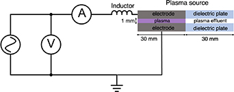
Figure 1. Schematic of the electrical circuit.
Download figure:
Standard image High-resolution imageFigure 2 shows the plasma source, feed gas lines and fluid setup. We used helium (Air Liquid, 99.999%) with and without controlled amounts of water vapor. The helium and humidified helium flow rates were controlled by mass flow controllers (MKS 1179 C). A simple thermostatic glass bubbler was used to humidify the He stream. The bubbler was kept inside a temperature-controlled bath (Thermo Scientific RTE 740) set at  . The gas line downstream of the bubbler was kept at
  with a heating tape to avoid any condensation of water vapor. To establish the humidity level, a calibration experiment was performed by weighting the water in the bubbler before and after helium was flowed inside for different flow rates and times. Liquid flow in the microfluidic devices was imposed from a distilled water (DW) reservoir by a syringe pump (New Era NE4000). Details on the design and operation of the microfluidic devices are presented in section 3.

Figure 2. Plasma feed gas setup and fluidic setup. The helium is humidified using thermostatic glass bubbler.
Download figure:
Standard image High-resolution image2.2. Plasma dissipated power
Plasma power dissipation (PPD) is one of the most fundamental and important plasma parameters and is frequently one of the first fairly complex measurements performed when using and/or developing a novel plasma source. The PPD measurement contains key information about the discharge state. However, PPD measurements can easily be inaccurate and special care must be taken when achieving such electrical diagnostics [29], especially when dealing with miniature NTP sources.
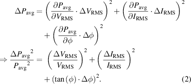
The average power dissipated during one electrical period is defined as:
where T is the period,  the time varying voltage and
  the time varying current. For a sinusoidal voltage waveform and a linear current response, the average power is:

where  is the root mean square voltage,
  is the root mean square current, and
  is the phase angle between the current and voltage. This phase angle,
  , arises from the load impedance to which the voltage is applied:
  . An error analysis of equation (1) leads to:
The last term of equation (2) contains  , whose value increases rapidly when the phase angle is close to
  . This can become problematic when measuring the delivered power to a highly capacitive load like miniature plasma sources. To overcome this challenge, Hoffmann et al [26] proposed, in the context of an atmospheric NTP source, to use a simple coupling network consisting of only an inductor. A non-ideal inductor, like the one used for the impedance coupling in this publication, has a resistivity. This resistive behavior comes from two sources: the non-zero resistance of the wires from which the inductance is made and the heating of the inductor's material through magnetic loss. As current is flowing through the resistive part of the impedance, power is dissipated. Hence, to isolate the power dissipated in the plasma discharge, the value of the resistive part of the inductor,
  , needs to be known. Figure 3 shows the equivalent circuit representation of the device with (on) and without (off) plasma. In the off configuration, power is only dissipated in
  . The quickest way to determine the value of
  is probably to measure the power dissipation without ignited plasma (off configuration). The relation between the power and
  will then be
  , where
  is the measured RMS current without a plasma discharge (off configuration) and
  the corresponding power. From this, the power dissipation in the discharge can be deduced by the subtractive method [30]:


Figure 3. Equivalent circuit of the plasma source with (on) and without (off) plasma discharge. When no plasma is ignited (off), the plasma source acts as a capacitor,  , and no power is dissipated in the plasma source. When plasma is ignited (on), power is dissipated in the discharge and the plasma source is represented as a capacitor,
  , in series with a resistor,
  .
.
Download figure:
Standard image High-resolution image
 is found by the regression of
  ,
,  and
and  are the RMS voltage and current with the plasma ignited (off configuration).
3. Microfluidic coupling
The difficulty in combining plasma sources with microfluidic devices arises from the special properties of liquids when manipulated in small volumes. In microfluidic regimes, the capillary forces play an important role: if not adequately confined liquids tend to spread inside small openings. Hence, creating an opening to allow interaction between liquid circulating in a microfluidic device while avoiding liquid infiltration in the plasma channel poses a challenge. The following presents how the plasma source was combined to a microfluidic device. The proposed plasma-microfluidic coupling enables creating a plasma-liquid interaction zone at a desired position in a controllable and reproducible manner.
3.1. Hydraulic resistance, flow rate and pressure in microfluidic devices
The microfluidic devices developed for the proposed plasma-microfluidic coupling have two main objectives. The first one is to allow liquid circulation for plasma treatment and the second is to obtain high control on the position of the plasma-liquid interaction zone. The liquid circulation is made possible by imposing a flow rate,  , while the position of the plasma-liquid interface is controlled by adjusting the pressure,
  , in the microfluidic channels. These two parameters,
  and
and  , are connected by the Hagen-Poiseuille law [31]:

where  is the fluidic resistance of the microfluidic channel and
  is the pressure variation across this channel. Equation (4) is interpreted as follows: imposing a flow rate
  in a channel of fluidic resistance
  leads to a pressure drop across the channel of
  . A strong analogy exists between the Hagen-Poisseuille law and Ohm's law,
  , that connects the voltage drop across a resistance (
 ) to the current flowing through it (
 ) by the electrical resistance of the wire (
 ).
).  can be customized by changing the geometry of the microfluidic channel. For example, a cylindrical channel has a fluidic resistance given by
  , where
  is the circulating fluid viscosity,
  is the length of the channel and
  is the radius of the cylindrical cross section. The latter equation shows that one can impose
  at a certain Q by controlling
  .
.
3.2. Microfluidic devices design
Figure 4 presents a simple schematic of the plasma microfluidic coupling. The plasma zone is ignited on top of the microfluidic device which consists of three main channels. The first one, on the left, is connected to a liquid reservoir and has a hydraulic resistance  . The second, on the right, is connected to a syringe pump and has a hydraulic resistance
  . In between them, a third channel, that will be called the chimney, allows contact between the plasma zone and the liquid circulating in the microfluidic device. Because of small channel sizes in the microfluidic device, capillary forces are significant. Without adequate control, the circulating water in the microfluidic device would creep inside the plasma channel and lead to changes in the plasma properties making it almost impossible to obtain reproducible experiments. Moreover, exposing the surface of the device to a plasma discharge increases its surface hydrophilicity, which tends to maximize capillary pressure. If this effect is not considered at the design stage, flow will spill out of the microchannel via capillary action and disrupt the device functioning. To avoid such problem, the microfluidic devices are designed to control the position of the liquid interface at the plasma channel. This is achieved by controlling the pressure under the liquid interface such as to offset capillary pressure, also known as Laplace pressure. The capillary pressure is given by
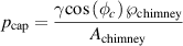

Figure 4. Plasma-microfluidic coupling. The liquid interface height, h, can be controlled by varying the  through the flow rate Q and/or the hydraulic resistance
  .
.
Download figure:
Standard image High-resolution imagewhere  is the liquid surface tension,
  is the contact angle between the liquid and the microfluidic device's walls,
  is the perimeter of the chimney and
  is cross section area of the chimney. The hydrodynamic pressure, the pressure drop associated to Hagen-Poiseuille's law, is given by:

where Q is the flow rate of the circulating liquid and  is the fluidic resistance of the channel between the liquid reservoir and the chimney for water. The gravitational pressure that originates from the liquid column's weight of the chimney is given by:

where  is the liquid density,
  is the gravitational acceleration and
  is the height of the liquid chimney. The liquid reservoir and the plasma channel are at atmospheric pressure,
  . At the bottom of the chimney, the pressure is given by:
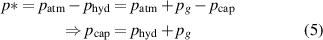
where all pressure values,  ,
,  ,
,  and
and  are positive-definite. From equation (5), we can deduce two regimes of operation. When
  , the capillary forces are dominant, and a liquid chimney exists. In this regime, only liquid is flowing in the microfluidic channel. This first regime is illustrated in figure 5(a). When
  , the hydrodynamic pressure combined with the gravity is dominant and no liquid chimney exists. In this case, both liquid and gas are flowing in the microfluidic device which offers a second regime of operation. This second regime is illustrated is figure 5(b) and will be further discussed in section 5.2. Note that in this multiphase regime, no liquid chimney exists and the gravitation pressure,
  , is of course zero. We keep the term
  in
in  for generality only. The microfluidic device is designed to control
  through
  at a desired liquid flow rate
  .
.

Figure 5. Schematic of the two operation modes of the microfluidic devices. (a) Single-phase flow ( ). (b) Multiphase flow (
 ).
).
Download figure:
Standard image High-resolution imageIn microfluidic, a T-junction is a junction of three channels and is probably one of the most common junctions. Figure 6(a) shows the schematic of a T-junction. T-junctions can be used to create a flow composed of two different liquids (such as water and oil), or a flow of one liquid and one gas (such as water and air). In a T-junction where the flow rates  and
and  are imposed, it is possible to predict the size of the bubbles or droplets formed by each fluid based on the proprieties of the fluids, the geometrical sizes of the T-junction and the values of
  and
and  [32]. These types of bubble formation experiments are well known and have been extensively studied by the microfluidic community. The junction that enables the coupling between the microfluidic devices and the plasma channel in our system resembles the just mentioned T-junction at one key difference: only one flow rate is imposed,
  in figure 6, and the value of
  and
and  will change depending on the value of
  . Hence, even if models exist to predict the gas–liquid or liquid-liquid bubble formation in a T-junction, they cannot be directly applied to our device.

Figure 6. A T-junction. (a) Imposed flows in the channels. (b) Fluidic resistance of the different channels.
Download figure:
Standard image High-resolution imageIn the complete plasma-microfluidic platform, the plasma source is positioned on top of the microfluidic device with the plasma channel aligned with the opening of the microfluidic device (see figure 5). A glass plate is then added above the plasma channel and the electrodes. The opening of the microfluidic device that creates the interaction between the liquid and the plasma generated reactive species can be placed at different positions. Figures 7(a) and (c) shows the opening (in the center of the red circles) directly under the plasma active zone. In (c), a plasma is ignited. In (b), the opening is positioned in the plasma effluent zone, 3 mm from the end of the active plasma zone. Hence, the position of this liquid interaction zone can be modified to study the spatial evolution of the plasma chemistry and its interaction with liquid.

Figure 7. Plasma source electrodes on top of the microfluidic device. In (a), the opening of the microfluidic device is positioned under the plasma active zone while in (b), the opening is in the plasma effluent. In (c), the plasma is ignited, and the opening is under the plasma active zone.
Download figure:
Standard image High-resolution imageThe microfluidic devices are designed in a CAD software (Fusion 360) and are 3D printed with a 27-micron resolution printer (Pico 2 HD, Asiga, Australia) using UV sensible resin (GR1-clear resin—Pro3Dure—A1000300).
4. Plasma-liquid interaction and H2O2 concentration assay
Liquid samples were plasma treated with the plasma-microfluidic platform and the liquid was diagnosed with a hydrogen peroxide concentration colorimetric assay. For the plasma treatments, the microfluidic devices were operated in the multiphase flow regime with DW as circulating liquid. For each experiment, the plasma dissipated power, the plasma feed gas humidity and the flow rate imposed by the syringe pump was kept constant for the treatment duration. At the end of the plasma treatment, the concentration of  in the liquid was determined colorimetrically. A solution of 2.5 g of titanium oxysulfate (
 ) in 100 ml of 2 M sulfuric acid solution was used to produce pertitanic acid, which is yellow in color, when reacting with
  . In 96-well plate, 160 μl of plasma treated liquid was mixed with 80 μl of the titanium oxysulfate solution and 40 μl of 30 mM sodium azide solution (for stabilization of the solution). The absorbances of the samples were measured on a Tecan Infinite 200 PRO plate reader at 407 nm. Calibration of the absorbance was achieved by replacing the plasma treated solution with solutions of
  of known concentration. Figure 8 shows the data and calibration curve for the measurement of
  concentration. Detection of
  through titanium oxysulfate is typically used for solution of
  of higher concentration than the one analyzed in this manuscript. This explains the significant uncertainty on the measurements. Nevertheless, the method was found sufficient to observe key trends on the
  concentration variation for different experimental parameters.

Figure 8.
 concentration of the samples function of the absorbance. The absorbance of samples of known concentration were measured for calibration.
Download figure:
Standard image High-resolution image5. Results and discussion
5.1. Power measurements
Figure 9 shows power measurement results from the method presented in section 2.2. The red dots represent the power dissipation without ignited plasma (off configuration). As previously mentioned, when no plasma is ignited, the power is dissipated almost exclusively in the resistive part of the coupling inductor,  . This explains the quadratic behavior of the dissipated power with the current (
 ). The red line represents the quadratic regression of the power with the current and the black and blue dots represent the power dissipated both in the plasma discharge and the coupling inductor (on configuration). With the regression and the total dissipated power, the PPD is calculated with equation (3). In figure 9, the black and blue dots represent the total dissipated power with a plasma-forming gas of pure helium and with a plasma-forming gas of pure helium mixed with an admixture of
  of 2100 ppm respectively. Both for pure helium and humidified helium, the point of minimal power is taken slightly after a visible plasma ignition and the point of maximal power is taken slightly before the transition to an arc plasma. Hence, we see that higher power density is needed to ignite the plasma in humidified helium. Analogously, humidified helium can hold a higher power density before transitioning to an arc discharge.

Figure 9. Power dissipation with and without an ignited plasma function of the RMS current. The power dissipated in the plasma discharge is given by the difference between the red curve and the power with an ignited plasma.
Download figure:
Standard image High-resolution image5.2. Microfluidic device operation
Liquid circulation in the microfluidic devices is possible in two principal modes of operation. The first one is a single-phase flow: only liquid is flowing in the microfluidic channels. In this regime, the microfluidic device's geometry and the liquid flow rate are chosen to bring plasma-liquid interface at a fixed position. Figure 10 shows pictures of tap water with food coloring (for better image contrast) flowing in a 3D printed microfluidic device in this single-phase liquid flow. In (a), the gas–liquid interface is held at the upper limit of the microfluidic device, while in (b) and (c) the gas–liquid interfaces are at lower positions. In figure 10, the height of the gas–liquid interface is controlled only by changing the imposed liquid flow rate in the microfluidic device. The second mode of operation is a multiphase flow. In this regime, both gas and liquid are circulating in the microfluidic device. Multiphase flow is achieved at higher flow rate than single-phase flow when  in equation (5). Figure 11 shows pictures of the multiphase flow at three different stages of the gas bubble formation in the microfluidic device. In (a), a gas bubble start forming in the fluidic channel. The bubble grows and elongates as seen in (b) until it is squeezed on the device's wall and liquid flows again as seen in (c). From there, the process repeats itself and another bubble starts to be formed. In this second mode of operation the ratio between gas and liquid that circulates in the microfluidic channels can be controlled by the fluidic resistance of the channel between the liquid reservoir and the opening of the device (
 of figure 6) or by the flow rate that is imposed in the microfluidic device (
 of Figure). The multiphase flow offers two key advantages. The first one is operation stability. An exact control of the gas–liquid interface like in the single-phase flow is particularly sensitive to changes such as flow rates or contact angle. Small instabilities can lead to liquid being dragged in the plasma channel which is strongly undesired as previously mentioned. The second advantage of the multiphase flow is the increased transport of plasma-generated reactive species compared to the single-phase regime. Indeed, the formation of the water droplets in the multiphase flow increases the diffusion transport in the droplets through convection and recirculation movement [33] while these recirculation movements do not take place in the single-phase flow.

Figure 10. Pictures of a microfluidic device operated in the single-phase flow. The height of the liquid interface is varied by changing the flow rate. The black arrows point to the position of the air-liquid interface.
Download figure:
Standard image High-resolution image
Figure 11. Pictures of a microfluidic device operated in the multiphase flow. Pictures (a)–(c) shows the different steps of the formation of the bubble in the microfluidic device.
Download figure:
Standard image High-resolution imageTo explain and predict the gas–liquid flow formation in the microfluidic device, we developed a mechanistic model that describes the liquid droplet-gas bubble train formation. This model enabled us to design the microfluidic device and interpret the key experimental observations.
5.2.1. Hypothesis for the bubble formation.
In our microfluidic device, fluid 1 of figure 6 is water while fluid 2 is air and the imposed flow rate by the syringe pump would be  . In the following, we approach the problem with Onsager's variational principal [34–36], which consists of minimizing the Rayleighian. The latter being the sum of the rate of energy dissipation in the system divided by two and the rate of change of the interfacial free energy. We know from experimental results that at low values of
  , only water is flowing in channel 3. It is the first flow regime, when
  . The power dissipated to impose this flow, which originates from viscous forces, before the T-junction is
  , where
  is the fluidic resistance of channel 1 for water. For higher values of
  we see experimentally that both water and air is flowing in channel 3. It is the second regime, when
  . The power dissipated by the system to impose this multiphase flow before the T-junction is
  , where
  is the fluidic resistance of channel 2 for air. The last approximation is applied because the viscosity of air is 2 orders of magnitude smaller than the one of water and because in our microfluidic device, channel 1 is much longer than channel 2 making
  negligible. For similar arguments, the power dissipated by the system for the flow in channel 3 can be approximated by
  , where
  is the fluidic resistance of channel 3 for water and
  is the fluidic resistance of channel 3 for air. The production of an air bubble in the channel also comes at an energy cost because of the formation of an air-water interface. The variation of the interfacial free energy for the formation of this interface is given by
  , where
  is the surface tension of water and
  is the time variation of the air-water interface area. For a channel of perimeter
  and a cross section area of
  , the power needed to create the air-water interface is given by
  . Hence the Rayleighian of the system is given by:
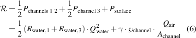
For the experimentally used flow rates and for the microfluidic channel sizes both terms  of equation (6) are of similar orders of magnitude in value. The system will tend to minimize the Rayleighian
  under the imposed constraint
  :
:
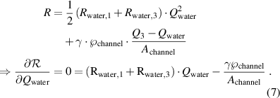
From equation (7) we can reduce the flow rates that minimize the power consumption:
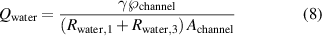
In figure 12, we can see qualitatively that at higher imposed flow rates ( ), with all other parameters kept constant, more air is dragged in channel 3 (
 ) as predicted by equation (9). Furthermore, we observed experimentally that using liquids with different surface tensions lead to a change in the average values of
  and
and  . We compared the bubble formation using water as fluid 1 (
 mN m−1) with using a solution of 70% ethanol in water as fluid 1 (
 mN m−1). We observed a higher flow rate of air with the ethanol solution as predicted by equation (9).

Figure 12. Gas–liquid flow at four different flow rates. At higher imposed flow rate, more air is dragged into the channel.
Download figure:
Standard image High-resolution imageDividing equation (8) by equation (9), we obtain the liquid droplet-gas bubble volume ratio predicted by the microfluidic model:
where  Using figure 12, we can determine this liquid droplet-gas bubble volume ratio (
 ) for the four different flow rates investigated. These experimental data are reported in figure 13 together with the best fit obtained with equation (10). An excellent fit can be obtained. The model adequately predicts the change of liquid droplet-gas bubble volume ratio as a function of the imposed flow rate (
 ). The fitted k value is
  ml min−1. This value can be compared to
  ml min−1, the value predicted by the model, with the geometrical sizes of the microfluidic device that was used to produce the multiphase flow in figure 12.
  and
and  differ by about one order of magnitude which is satisfactory considering the simplicity of the microfluidic model.

Figure 13. Liquid droplet-gas bubble volume ratio observed at different imposed flow rates and fitting curve given by equation (10). For each flow rate the volume of 5 liquid droplets and 5 gas bubbles were averaged to compute the volume ratio. The error bars are given by the standard deviation of the volumes with error propagation of the droplet-gas bubble volume ratio.
Download figure:
Standard image High-resolution imageThis analysis of the microfluidic model remains limited as our theoretical approach that leads to equations (8) and (9) has not yet been compared with sufficient experimental data. Our simplified model also conspicuously neglects corner flow leakage around air bubbles during their formation [36] which might partially explain the discrepancy between  and
and  . However, the simplified model based on the previously stated assumptions infers accurately that the formation of a multiphase air-water flow arises from a competition between the change of free energy associated with creating an air-water interface and the energy dissipation associated with imposing a water flow in a microfluidic channel. With this model, we were able to design the microfluidic devices to accurately control the gas bubble-water droplet volume ratio and velocity profile in the microfluidic device.
5.3. H2O2 concentration assay
The effect of the variation of feed gas humidity and PPD on  production and transport in the circulating liquid of the microfluidic device were studied (figures 14 and 15). For each of them, the concentration of
  was compared for the opening of the microfluidic device directly under the active plasma and under the plasma effluent, 3 mm downstream of the active plasma, as seen on figure 8.

Figure 14.
 concentration function of the humidity in the feed gas.
Download figure:
Standard image High-resolution image
Figure 15.
 concentration function of the power dissipated in the plasma discharge.
Download figure:
Standard image High-resolution image
Figure 14 illustrates the variation of  concentration in the plasma treated liquid when the concentration of humidity in the feed gas is changed. For each point on this graph, the power dissipated in the plasma was kept constant at
  W. The final concentration of
  in the treated liquid increases with the humidity in the feed gas. Since the main production path of
  is through the combination of two
  radicals [37], a higher production of OH radicals leads to a higher production of
  . As humidity is increased in the plasma feed gas, more
  radicals are formed by dissociation of water molecules through electron-impact reaction (
 ) which in turn leads to higher
  concentration in the liquid. Furthermore, the presence of
  is systematically higher for the interaction point in the plasma effluent. This is explained by two main reaction pathways. Firstly, as mentioned, because
  radicals' recombination is the main formation pathway of
  and
and  radicals quickly recombine in the plasma effluent. Secondly, because the main destruction pathway of
  is through an electron-impact reaction (e +
  ), which no longer takes place in the plasma effluent. When the plasma is operated in pure helium, i.e. with a
  ppm impurity concentration of humidity, the final
  concentration in the treated liquid is lower than the detection limit, suggesting that
  radicals are mainly formed from the dissociation of water molecules originally in the plasma-forming gas and not from additional humidity added by evaporation of water circulating in the microfluidic device.
Figure 15 shows the variation of  concentration in the plasma treated liquid for a change of plasma dissipated power. Both with the opening of the microfluidic device under the active plasma and under the plasma effluent, the increase of power dissipated in the plasma leads to an increase of
  concentration in the treated liquid. This could be explained by two reaction pathways. The first one is the increased evaporation of the water circulating in the microfluidic device when the power, and hence the gas temperature, is increased. However, as mentioned, result of figure 14 suggests that the effect on
  concentration of evaporation from the water in the microfluidic device is low. The second pathway, and the most probable, is an increased dissociation rate of water molecules with higher plasma power. Higher power thus leads to higher production of
  radicals by the plasma which in turn leads to a higher
  concentration in the plasma, plasma effluent and in the treated liquid.
6. Conclusion
In this manuscript, the COST reference plasma jet was for the first time coupled with microfluidic devices. The interface between the plasma channel and the circulating liquid in the microfluidic device was controlled by engineering the microfluidic channels' geometry and the imposed flow rate by a syringe pump. The use of direct 3D printing for fabrication of microfluidic devices makes their prototyping fairly easy and rapid. The proposed plasma-microfluidic coupling opens the way to new plasma-liquid interactions studies. The efficient control of liquids on a small scale enables the interaction between liquid and plasma-generated reactive species with a high spatial resolution. We know that for miniature NTP jet sources, plasma chemistry is highly spatially dependent, i.e. reactive species concentration varies greatly in the plasma jet and its surroundings. The proposed method could help understand how this spatial variation can influence the chemistry of liquid in contact with plasma jets. We developed microfluidic devices that allow stable operation of the platform and we think that the formation of the liquid droplet-gas bubble train in the multiphase flow is probably the best approach to maximize the transport of reactive species in the microfluidic devices and to study the plasma-generated species transport pathways at the gas–liquid boundary. Also, controlling the flow rate in the microfluidic device also means one can control the velocity of the circulating liquid. This can be of high interest for liquid reaction kinetic analysis since by controlling the velocity, the reactions' time delays can be easily coupled to liquid path distances in the microfluidic device. Furthermore, the proposed plasma-microfluidic platform could open the way to the coupling of existing microfluidic device, used for biological applications such as cancer treatment studies, with different NTP sources such as the COST-Jet, but also NTP sources developing long plasma column [38] or micro-sized plasma plume [39]. We think that understanding and tailoring the formation and transport pathways of plasma generated reactive species will play a key role in future research of NTP for biomedical applications and that the combination of NTP sources with microfluidic could be of help in these studies.
Acknowledgments
The authors acknowledge the financial support from the Fond de recherche du Québec, the Natural Sciences and Engineering Research Council of Canada (including Grant Nos. RGPIN-06838 and RGPIN-06820), Gerald Hatch Faculty Fellowship from McGill University and the TransMedTech Institute through its main financial partner, the Apogee Canada First Research Excellence Fund.
Data availability statement
All data that support the findings of this study are included within the article (and any supplementary files).