
Abstract
Here, we compare the ionization region model (IRM) against experimental measurements of particle densities and electron temperature in a high power impulse magnetron sputtering discharge with a tungsten target. The semi-empirical model provides volume-averaged temporal variations of the various species densities as well as the electron energy for a particular cathode target material, when given the measured discharge current and voltage waveforms. The model results are compared to the temporal evolution of the electron density and the electron temperature determined by Thomson scattering measurements and the temporal evolution of the relative neutral and ion densities determined by optical emission spectrometry. While the model underestimates the electron density and overestimates the electron temperature, the temporal trends of the species densities and the electron temperature are well captured by the IRM.
Export citation and abstract BibTeX RIS

Original content from this work may be used under the terms of the Creative Commons Attribution 4.0 license. Any further distribution of this work must maintain attribution to the author(s) and the title of the work, journal citation and DOI.
1. Introduction
Magnetron sputtering [1] is a physical vapor deposition technique [2] that has become the deposition process of choice for a wide range of industrially relevant coatings [3, 4]. This technique has developed rapidly over the past decades, driven by an increasing demand for high-quality functional thin films and coatings for an ever-increasing range of applications [1, 3]. In the magnetron sputtering discharge a dense plasma is trapped in the cathode target vicinity by a static magnetic field forming an ionization region (IR). When driven by dc voltage or current, the sputtered species that reach the substrate constitute almost only neutral atoms. However, it can be beneficial for the resulting deposited films to have the flux onto the substrate to also contain ions of the sputtered species. Therefore, among the important advances of the magnetron sputtering technique in recent decades, is the possibility of increased ionization of the sputtered film-forming species [4–6], which has turned out to become a game-changer for thin-film deposition by magnetron sputtering [7].
High power impulse magnetron sputtering (HiPIMS) is one approach to create a highly ionized flux of the film-forming material onto the substrate. High voltage pulses of short duty cycle (typically 0.5%–5%) are applied to the cathode target and lead to a high peak discharge current density (0.5–10 A cm−2) and therefore to a high electron density ( cm−3) within the magnetic trap [8–10]. Consequently, the species sputtered from the target are ionized as they pass through the dense plasma of the IR. When the film-forming material is ionized, the ion bombarding energy can be controlled by biasing the substrate [6, 7], which provides an additional parameter for process development. The metal ions provide efficient energy and momentum transfer to the growing film surface which makes a deposition at lower substrate temperatures possible, while still achieving the desired film properties [11]. The film-forming species are then primarily incorporated at lattice sites resulting in films exhibiting much lower compressive stress, while noble gas trapping at the interstitial sites is avoided [7, 12].
One application for magnetron sputtering is the fabrication of tungsten thin films. Sputter-deposited tungsten thin films exhibit two phases, the equilibrium  W (A2 bcc) and the metastable
  W (A15 cubic) phases. HiPIMS-deposited tungsten films are denser, exhibit smaller grains and better adhesion [13–15] in addition to higher hardness, higher Young's modulus values, and smoother surfaces [13, 16, 17]. This is well demonstrated by Shimizu et al [15] who reported stress-free, unstrained single phase
  W thin films, deposited by applying a synchronized substrate bias to selectively increase the energy of the metal population of the ion bombardment.
To understand the discharge processes that lead to the desired film properties in deposition experiments, one can resort to plasma characterization. For example, Ryan et al employed Thomson scattering measurements, to resolve the temporal evolution of the electron density and electron temperature in a HiPIMS discharge with a tungsten target [18, 19]. In addition, Ryan et al measured the electron densities and temperatures using a Langmuir probe, which showed a good agreement with before-mentioned results from the Thomson scattering measurements [20]. Furthermore, the temporal evolution of certain emission lines from the heavy species were recorded using optical emission spectrometry (OES) [19].
A different methodology to characterize plasma discharges is by modelling. The IR model (IRM) is a semi-empirical volume-averaged global model of the plasma chemistry of a pulsed magnetron sputtering discharge [21, 22]. Recently, a tungsten reaction set and related surface processes were incorporated in the IRM and applied to study a HiPIMS discharge with a tungsten target as the discharge voltage was varied [23]. It was seen that the contribution of the W+ ions to the total discharge current at the target surface increases with increased discharge voltage for peak current densities  in the range from 0.33 to 0.73 A cm−2 [23]. Furthermore, the ionization probability of the sputtered tungsten increases, while the back-attraction probability decreases, with increased discharge voltage and peak current density.
Here, the objective is to compare the calculated IRM results with measurements. For this, we model three discharges that were characterized experimentally by Ryan et al [18, 19]. This allows us to compare the measured plasma parameters, in particular the temporal evolution of the electron temperature and electron density (from Thomson scattering measurements) and the temporal evolution of the neutral and ion densities of the working gas and sputtered species (from OES), to the model results.
In section 2 a brief overview of the experimental setup is given followed by a brief summary of the IRM in section 3. The results of the IRM calculations are discussed and compared to the experimental findings in section 4. A summary is given in section 5.
2. Experimental apparatus and method
The experiments were carried out in a custom-built cylindrical vacuum chamber (height 500 mm and diameter 450 mm) made of stainless steel. The discharge was driven by a SINEX 3 pulser unit (Chemfilt Ionsputtering A.B., Sweden). A 150 mm diameter tungsten target was mounted on a VTech 150 series unbalanced magnetron assembly (Gencoa Ltd., United Kingdom). Argon at a pressure of 1.6 Pa was used as the working gas. This is a somewhat higher working gas pressure than typically used in HiPIMS operation, but high density and low electron temperature conditions are favourable for the (peak) signal-to-noise ratio of the Thomson scattering spectrum. The pulses were 50 µs, 100 µs, and 200 µs long, and the repetition frequency was 50 Hz. For the three cases, an average discharge power  was maintained at 400 W. The discharge voltage and current waveforms measured for the three cases are shown in figure 1. Note that both the discharge voltage and the discharge current vary with time as the SINEX 3 pulser unit has a smaller storage capacitor compared to more modern pulser units [24, 25]. Figure 1(a) shows that the discharge voltage exhibits a similar temporal behavior regardless of the pulse length. The discharge current waveform (figure 1(b)) exhibits a spike in the beginning of the pulse followed by a monotonic decrease until the voltage is cut off. The discharge voltage is slightly higher (about 11% higher 10 µs into the pulse) when the pulse length is shorter. We see in figure 1(b) that the peak discharge current is higher for the shortest pulse length of 50 µs, while the discharge current for the longer pulses (100 µs and 200 µs) exhibits the same peak current and are almost identical until they are cut off.

Figure 1. The temporal evolution of the discharge (a) voltage  and (b) current
  . The argon working gas pressure was 1.6 Pa and the target was made of tungsten 150 mm in diameter.
Download figure:
Standard image High-resolution imageThomson scattering measurements were applied on the discharges to determine the temporal variation of the electron temperature and the electron density. A Nd:YAG laser operated at the second-harmonic wavelength (532 nm) was the radiation source. The laser energy per pulse was  240 mJ, the pulse duration 5 ns, the repetition rate 10 Hz, and the beam divergence 0.5 mrad. The laser beam was focused by a 1 m focal length lens to create a beam diameter of ∼0.25 mm at the measurement location, on a spot 10 mm above the racetrack, in the magnetic trap region (r = 41 mm, z = 10 mm), where the magnetic field strength was 33 mT [19], as shown schematically in figure 2. The beam path was in the plane of the target surface and the laser electric field was linearly polarized in the direction perpendicular to the plane of the target surface. The scattering volume was 0.15 mm in diameter and 3 mm long. The scattered light was collected by a lens (75 mm in diameter and focal length f = 200 mm) positioned at 90∘ with respect to both the laser propagation and polarisation axes in order to maximise the Thomson scattering differential cross-section. An image of the detection volume was presented onto the entrance slit (0.30 mm × 6 mm (the slit length was parallel to the laser propagation axis)) of a triple-grating spectrometer (TGS (Horiba T64000)). The spectrometer was configured in the double-subtractive configuration to attenuate the wavelength region 531.5–532.5 nm using a mask, a notch filter, to remove the stray laser light and Rayleigh scattering signals. An intensified charge-coupled device camera (Andor iStar DH320T-18U-A3) was used to record the spectra in two-dimensions. The wings of the Thomson spectra were fitted by either a single or double-Gaussian curve, corresponding to a Maxwellian or bi-Maxwellian electron velocity distribution function, respectively, to obtain the electron density and electron temperature. The system was calibrated for absolute density measurements using Rayleigh scattering from room temperature argon gas after each Thomson scattering measurement. The Thomson scattering signal was accumulated from 600 pulses for each time-resolved data point. From the Thomson scattering measurement, the temporal evolution of the absolute electron density and electron temperature was constructed.

Figure 2. A schematic showing the magnetic field from an unbalanced planar magnetron assembly with a 150 mm diameter tungsten target, and the measurement position above the racetrack (r = 41 mm and z = 10 mm). The magnetic null position is r = 0 mm and z = 61 mm.
Download figure:
Standard image High-resolution imageTime-resolved OES measurements were performed in the magnetic trap region (r = 41 mm, z = 10 mm (see figure 2)) by Ryan [19] to provide information on the species composition in the discharge. This involved measuring the intensity of selected line emissions. These lines represent the various species: Ar I (751.47 nm), Ar II (480.60 nm), W I (361.75 nm), and W II (361.38 nm). The lines were chosen based on their relatively strong intensity and their large Einstein coefficient for spontaneous emission. Moreover, care was taken that they did not overlap with other significant transition lines. Therefore, the emission intensity is assumed to be representative of the instantaneous density of the upper excited level of the transition. The OES results presented in this article are displayed as relative intensities, where each data point in a temporal profile of line emission intensity is normalised by the maximum intensity measured in that particular time series. For each time-resolved data point the acquisition time was 10–20 s (500–1000 pulses). The line emission intensity was calculated by fitting a Gaussian curve to the peak and then calculating the area under the curve. More details of the experimental setup and methods are given elsewhere [19].
3. The IRM
The IRM is a semi-empirical volume-averaged discharge model that requires inputs from an experimental discharge. These inputs are the discharge voltage and current waveforms, as well as the working gas pressure, and an estimated size of the IR [21, 22]. The IRM has been under development for well over a decade and has been applied in a number of studies to reveal the processes within a HiPIMS discharge [21–23, 26].
The IR in the model is assumed to be an annular cylinder with outer radius  , and inner radius
  . It resides on top of the circular racetrack and has a height of
  , extending axially away from the target surface. For the studied discharges the parameters for the size of the IR are assumed to be:
  = 12 mm,
  = 57 mm, z1 = 2 mm, z2 = 33 mm. We explore how this choice of the dimensions of the IR influences the results in
In the model, we assume two electron populations, one cold population and one hot population. The majority of the electrons in the discharge are members of the cold electron population. They are created through volume reactions within the IR. This population essentially determines the electron density and the effective electron temperature. Hot electrons stem from secondary electron emission created by the ion bombardment of the cathode target. The electrons can gain energy either by being accelerated in the sheath or by Ohmic heating [22]. In each part, a fraction of the discharge power is dissipated [10], that is fed into the model via the discharge current and voltage waveforms. At the start of the simulation, we add an initial electron density of  m−3. In the
The temporal development of the heavy species densities is defined by a set of ordinary differential equations [22], involving rate coefficients for each of the electron populations. The rate coefficients are calculated assuming a Maxwellian electron energy distribution function [22]. The rate coefficients for the cold electron population are valid in a range from  –7 eV. The rate coefficients for the hot electron population are valid in a range from 200 to 1000 eV. This was shown to be a good approximation by comparison to the electron energy distribution calculated by the Orsay Boltzmann equation for ELectrons coupled with Ionization and EXcited states kinetics (OBELIX) model, which includes a Boltzmann solver [27]. The complete reaction set for the argon working gas and the tungsten discharge is listed in an earlier work [23], where the reaction set involving the tungsten discharge was discussed in detail, but the rate coefficients involving tungsten species are also listed in table 1.
Table 1. The reactions and rate coefficients used in the IRM involving tungsten, determined for both hot and cold electrons. The rate coefficients are calculated assuming a Maxwellian electron energy distribution function and fit in the range  –7 eV for cold electrons and 200–1000 eV for hot electrons.
| Reaction | Threshold (eV) | Rate coefficient (m3 s−1) | electrons | Reference |
|---|---|---|---|---|
(R1) e + W  W+ + e W+ + e | 7.864 |

| cold | [28] |

| hot | |||
(R2) e + W+
 W2+ + e W2+ + e | 16.35 |

| cold | [29] |

| hot | |||
(R3) Ar + W + W  Ar + W+ Ar + W+
|

| [30] | ||
(R4) Ar(4s'[1/2]0) + W  Ar + W+ + e Ar + W+ + e |

| |||
(R5) Ar(4s[3/2]2) + W  Ar + W+ + e Ar + W+ + e |

|
Not every necessary model parameter is possible to obtain experimentally. There are three parameters that are unknown a priori: (i) the ion back-attraction probability for the metal ions  and gas ions
  (it is assumed that
  as in previous studies [21–23]), (ii) the potential drop across the IR,
  , and (iii) the electron recapture probability r. For the latter, we assume r = 0.7, as it has been suggested by Buyle et al [31] that the electron recapture probability is typically between 65% and 75% for a planar magnetron sputtering discharge. This leaves two remaining parameters, that are found in a model fitting procedure. The best fit to the measured discharge current is determined by varying the fraction of the discharge voltage that drops across the IR f (with a resolution of
  = 0.01) and the back-attraction probability of an ion of the sputtered species during the pulse
  (resolution
  = 0.025). The model chooses values for the two parameters for which the discharge currents between the experiment and the model matches best.
An example fitting map is shown in figure 3 for the discharge with a 200 µs-long pulse. The blue zones in the fitting map (figure 3) indicate the combinations of  and
and  where the weighted square deviation of the discharge current is smallest, which is where the modeled discharge current resembles the experimental discharge current best. The resulting best fits to the discharge current waveform determined by the IRM
  for the 200 µs long pulse is shown with dashed lines along with the measured discharge current
  shown by solid lines in figure 4.
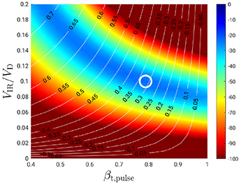
Figure 3. A fitting map showing the back attraction probability  versus
  for a discharge with a 150 mm diameter tungsten target, argon working gas pressure of 1.6 Pa, and pulse length of 200 µs. The white circles show where a well fitted discharge current waveform is observed. The white lines and the accompanying numbers indicate the ionized flux fraction.
Download figure:
Standard image High-resolution image
Figure 4. The temporal evolution of the measured discharge current ( ) and the model calculated discharge current (
 for a 150 mm diameter tungsten target, argon working gas pressure of 1.6 Pa, and 200 µs long pulse.
Download figure:
Standard image High-resolution image4. Results and discussion
The internal discharge parameters derived from the IRM for the HiPIMS discharges with a tungsten target are given in table 2. The ionization probability of the sputtered species αt is in the range from 0.89 to 0.81, the back-attraction probability  increases from 0.54 to 0.79, and the ionized flux fraction decreases from 0.65 to 0.32, as the pulse length is increased from 50 µs to 200 µs. Shorter pulse length increases the ionized flux fraction and lowers the back-attraction probability.
Table 2. Operation parameters, the pulse length  and the peak discharge current
  , and parameters derived from the modeling of a HiPIMS discharges with a tungsten target, the working gas rarefaction, the ionization probability αt, the back-attraction probability βt, the fractional voltage drop across the ionization region f, and the ionized flux fraction
  .
.
 (µs) (µs) |
 (A) (A) |
 (A cm−2) (A cm−2) | maximum degreeof rarefaction (%) | αt |

| βt |

|

|
|---|---|---|---|---|---|---|---|---|
| 50 | 263.2 | 1.49 | 69.4 | 0.89 | 0.61 | 0.54 | 0.10 | 0.65 |
| 100 | 206.5 | 1.17 | 65.1 | 0.83 | 0.76 | 0.74 | 0.10 | 0.39 |
| 200 | 205.2 | 1.16 | 64.8 | 0.81 | 0.79 | 0.79 | 0.10 | 0.32 |
The temporal evolution of the neutral particle densities for the 200 µs-long pulse is shown in figure 5. The cold ground state working gas argon atoms (denoted Ar (3p6)) dominate the discharge. However, their density decreases steadily with increased discharge current during the pulse, exhibiting a minimum which coincides with the peak in the discharge current. This is an indication of working gas rarefaction, a phenomena that has been observed experimentally to be rather significant in HiPIMS operation [32–36]. It is also seen that there is a sharp increase in the density of both the warm and hot argon atoms in the initial stages of the pulse. The maximum degree of working gas rarefaction, determined by adding all neutral argon atoms within the IR, and comparing them to the initial cold Ar density, is in the range 65%–69%. Figure 5 also shows that the ground state tungsten atom W0 density increases early in the pulse and becomes the second highest density species in the discharge for a short time early in the pulse. The metastable argon atoms exhibit more than an order of magnitude lower density.

Figure 5. The temporal evolution of the neutral particle densities for a discharge with a 150 mm diameter tungsten target, argon working gas pressure of 1.6 Pa, and 200 µs long pulse. The dashed vertical line indicates the termination of the pulse.
Download figure:
Standard image High-resolution imageFigure 6 shows the temporal evolution of the ion densities. The Ar+ ions dominate the ion densities only during the first few microseconds of the pulse. Early in the pulse the W+ ions take over as the dominating ions and remain dominating until the termination of the pulse. For much of the pulse duration and the afterglow the W+ ions exhibit roughly an order of magnitude higher density than the Ar+ ions. At the peak in the discharge current, the density of tungsten ions reaches a value of around  m−3 versus
  m−3 for the argon ion density. For all cases investigated, the Ar2+ ion density peaks around
  m−3, which is more than three orders of magnitude smaller than the W+ ion density. The W2+ ion density is roughly two orders of magnitude smaller than the W+ ion density. Note that the small bump seen in all ion densities at pulse-end in figure 6 is not due to a sudden increase in ion gain rates, but instead a result of a reduced ion loss rate from the back-attraction βt, becoming zero in the pulse afterglow, which consequently leads to a jump in ion density in the IR [37]. The model results for the temporal evolution for both neutrals and ions agree with the findings from our earlier modeling of a HiPIMS discharge with a tungsten target [23] as well as experimental observations [15]. Note that for the discharges explored in earlier studies the discharge voltage was maintained throughout the pulse, while in this current work the discharge voltage varies greatly through the pulse, as can be seen in figure 1(a).
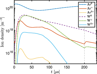
Figure 6. The temporal evolution of the charged particle densities for a discharge with a 150 mm diameter tungsten target, argon working gas pressure of 1.6 Pa, and a 200 µs-long pulse. For comparison the total argon neutral density (ground state and excited states) Ar0 and the neutral tungsten density W0 is also shown. The dashed vertical line indicates the termination of the pulse.
Download figure:
Standard image High-resolution imageThe temporal evolution of the discharge current composition at the target surface is shown in figure 7 for a 200 µs long pulse. The other pulse lengths have very similar compositions (not shown). Early in the pulse Ar+ ions dominate the heavy charged species in the discharge, before it is taken over by W+ ions. Initially argon ions bombard the target and sputter off metal atoms that are ionized and consequently return to the target and sputter off metal atoms again, and therefore, constitute a self-sputter recycling loop [38], where the tungsten atoms and ions, partially take over the role of the working gas argon atoms and ions as the pulse progresses. The fact that W+ ions dominate the discharge causes the secondary electron emission from the target to become very small (see  in figure 7), as the secondary electron emission yield is zero for W+ ions bombarding tungsten target.

Figure 7. The temporal evolution of the discharge current composition at the target surface for a discharge with a 150 mm diameter tungsten target, argon working gas pressure of 1.6 Pa, and 200 µs long pulse.
Download figure:
Standard image High-resolution imageFigure 8 shows the temporal profiles of the intensity of line emission, normalised by the peak number of counts for each line in a profile, from various species in the plasma discharge (Ar0, Ar+, W0 and W+) (dashed lines). The measurement was performed on a discharge formed with a 100 µs-long pulse and the average power was 400 W with a 50 Hz repetition rate, and the working gas pressure was 1.6 Pa. The intensity of the Ar0 line decreases, while the Ar+ emission intensity peaks at t = 20 µs, and the emission from both tungsten species increases. The figure also includes, for comparison and validation, the results of the model calculations (solid lines). The model results show a somewhat slower decay of the Ar0 density than observed experimentally (figure 8(a)). The 751.5 nm emission line from an argon atom is due to the decay from the 13.48 eV level in the 4p manifold to the 11.83 eV radiative level in the 4s manifold. We assume that electron impact excitation from the ground state dominates the excitation process. The reaction rate for electron impact excitation of the ground state argon atom is  , where
  is the excitation rate coefficient to the particular 4p state, which depends both on the electron density, the working gas pressure, and the electron temperature. We are aware that there is also some excitation from the metastable states into the 4s manifold. Earlier we have estimated the contribution of stepwise ionization from the metastable levels of the 4s manifold in HiPIMS operation to be as high as 15% [39], and we would expect a similar contribution to the excitation to the 4p manifold. Also, keep mind that there can be a decay from the 13.48 eV level to other levels of the argon atom. Similar arguments apply for the other measured lines from the heavy species used in this study. The peak in the Ar+ density appears roughly at the same time for the model calculation as determined experimentally, but the calculated Ar+ density decays somewhat faster than the measured density (figure 8(b)). The peak in the calculated relative W0 density appears somewhat earlier and decays much faster than the measured W0 density peak, as the measurements indicate that the W0 density remains high almost to the termination of the pulse, which is something that the model does not capture (figure 8(c)). The W+ ion emission intensity peaks roughly 30 µs into the pulse, and the model calculations agree with the measurements (figure 8(d)).

Figure 8. The temporal evolution of the relative optical emission from the various species (a) Ar0, (b) Ar+, (c) W0, and (d) W+, for 100 µs pulse length, argon working gas pressure of 1.6 Pa, and a discharge with a 150 mm diameter tungsten target. The experimental data is from Ryan [19], shown with dashed lines, and the IRM results are shown as solid lines.
Download figure:
Standard image High-resolution imageThe temporal evolution of the electron density and the electron temperature in a HiPIMS discharge with a tungsten target was determined experimentally using Thomson scattering [18–20]. The measured temporal evolution of the electron density from the Thomson scattering measurements is shown in figure 9. For the 50 µs long pulse the measured maximum electron density is  m−3 [18] (figure 9(a)), while for the longer pulses the measured peak value is
  m−3 (figures 9(b) and (c)).

Figure 9. The measured temporal evolution of the electron density and the calculated electron density for pulse length of (a) 50 µs, (b) 100 µs, and (c) 200 µs for a discharge with a 150 mm diameter tungsten target and argon working gas pressure of 1.6 Pa. The dashed vertical line indicates the termination of the pulse.
Download figure:
Standard image High-resolution imageThe measured temporal evolution of the electron density is compared to the calculated primary electron density in figure 9. Clearly, there is a discrepancy between the experimental and modelled electron density. The calculated electron density is always lower than the measured electron density. This discrepancy is up to a factor 4 during the peak for the 50 µs pulse length and somewhat smaller for 100 µs and 200 µs pulse length. However, it should be taken into account that the IRM is a simple global model with densities averaged over the entire IR volume, which is here assumed to extend 33 mm away from the cathode target, while the measurement is taken 10 mm from the target surface. Therefore, if we assume the electron (and ion) density to decrease with distance from the target surface, it is expected that the model calculations yield a smaller electron density than what is measured close to the target surface. Recent study by Dubois et al [40] determined, using Thomson scattering measurements, the variation in the electron density and electron temperature with distance from the target surface above the race track. The electron density was found to drop with distance from the target surface following a bi-exponential dependence. For pulse length of 70 µs, an argon working gas pressure of 1 Pa, a titanium target, and a peak discharge current of 40 A, the electron density 6 mm above the target surface was  m−3 and had fallen to half this value roughly 15 mm, and by about 70% roughly 25 mm above the target surface. This shows that a significant variation in electron density is to be expected within the IR.
Figure 10 shows the temporal profiles of the electron temperature within the magnetic trap for pulse lengths of 50 µs, 100 µs, and 200 µs. The electron temperature for the three discharges is similar during the overlapping pulse-on periods. The direct comparison of the calculated and measured electron temperature shows a discrepancy (figure 10). The calculated electron temperature is always significantly higher than the measured electron temperature. This again can be explained by the extension of the modelled IR, and the location of the measured volume, as the study by Dubois et al [40] indicates an exponential drop in the electron temperature with distance from the target surface. However, we like to point out that the features in the temporal evolution of the electron temperature are mostly captured by the model.

Figure 10. The measured temporal evolution of the electron temperature and the calculated primary electron temperature for pulse length of (a) 50 µs, (b) 100 µs, and (c) 200 µs for a discharge with argon working gas pressure of 1.6 Pa and a 150 mm diameter tungsten target. The dashed vertical line indicates the termination of the pulse.
Download figure:
Standard image High-resolution imageDespite the explainable differences between the experimental results and the model, we consider the model to reproduce the important trends in the electron temperature and the species density temporal evolution. Note that the objective of the IRM is to describe exactly these trends in HiPIMS discharges [21, 22]. The assumptions and necessary simplifications (e.g. it neglects spatial variation and uses an assumed EEDF) render the IRM considerably more efficient compared to e.g. particle-in-cell Monte Carlo collision simulations. This makes it possible to use the IRM for e.g. deposition process optimization [37, 41, 42], not possible with other modeling methodologies.
5. Summary
We have applied the IRM to explore a HiPIMS discharge with a tungsten target. Applying the IRM, the temporal evolution of the species densities and the internal discharge properties of the HiPIMS discharge can be determined. It is shown that Ar+ ions dominate the discharge current at the target surface in the initial stages of the pulse, but W+ ions take over early in the pulse and dominate the discharge current for the remainder of the pulse duration. The IRM calculation were compared to the experimentally determined temporal evolution of the electron density and electron temperature from Thomson scattering measurements and the temporal evolution of the heavy species determined by OES. The IRM captures the relative temporal evolution of the ions and neutrals of the working gas and sputtered species. However, we find that the model underestimates the electron density and overestimates the electron temperature, but captures well the trends of the temporal evolution of the electron temperature and density.
Acknowledgments
This work was partially funded by the Icelandic Research Fund (Grant No. 196141), the Swedish Research Council (Grant No. VR 2018-04139), the Swedish Government Strategic Research Area in Materials Science on Functional Materials at Linköping University (Faculty Grant SFO-Mat-LiU No. 2009-00971).
Data availability statement
All data that support the findings of this study are included within the article (and any supplementary files).
Appendix: Sensitivity analysis
The question that remains is if the discrepancy in the electron density and the electron temperature values is due to the choice of initial values or the assumption of the size of the IR, which is a somewhat arbitrary. Figure 11 shows a sensitivity analysis of the effect of the initial electron density on the temporal evaluation of the electron temperature. We compare the calculated electron temperature assuming initial electron density of  m−3, 1018 m−3, and 1019 m−3. For a lower initial electron density the initial peak in the electron temperature is somewhat higher, but after the initial peak the electron temperature is the same regardless of the initial value. For all cases the calculated electron temperature is well above the measured value. Therefore, the initial electron density does not have much influence on the calculated value of the electron temperature. A sensitivity analysis of the effect of the initial electron density on the temporal evaluation of the electron density is shown in figure 12. In all cases the calculated electron density is well below the measured value and the initial electron density does not have much influence on the overall results, except that a too high value can create an overshot in the first few µs. Figure 13 shows a sensitivity analysis of the effect of the size of the IR on the temporal evaluation of the electron temperature. We compare the calculated electron temperature for
  mm and
  %. In all cases the calculated electron temperature is well above the measured value. Therefore, the size of the IR does not have much influence of the calculated value of the electron temperature. Figure 14 shows a sensitivity analysis of the effect of the size of the IR on the temporal evaluation of the electron density. We show the results for
  mm and then when
  %. In all cases the calculated electron density is well below the measured value. Therefore, the size of the IR does not have much influence of the overall results. The choice of initial electron density or the size of the IR does not have a major influence on the overall results.
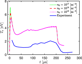
Figure 11. The temporal evolution of the electron temperature for pulse length of 200 µs for a discharge with a 150 mm diameter tungsten target and argon working gas of 1.6 Pa. The model results for the electron temperature are calculated assuming varying initial electron density.
Download figure:
Standard image High-resolution image
Figure 12. The temporal evolution of the electron density for pulse length of 200 µs, for a discharge with a 150 mm diameter tungsten target and argon working gas pressure of 1.6 Pa. The model results for the electron density are calculated assuming varying initial electron density.
Download figure:
Standard image High-resolution image
Figure 13. The temporal evolution of the electron temperature for pulse length of 200 µs for a discharge with a 150 mm diameter tungsten target and argon working gas pressure of 1.6 Pa. Sensitivity analysis where the electron temperature is calculated while varying the size of the IR,  mm and
  %.
%.
Download figure:
Standard image High-resolution image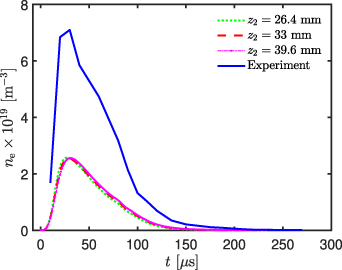
Figure 14. The temporal evolution of the electron density for pulse length of 200 µs for a discharge with a 150 mm diameter tungsten target and argon working gas pressure of 1.6 Pa. Sensitivity analysis where the electron temperature is calculated while varying the size of the IR,  mm and
  %.
%.
Download figure:
Standard image High-resolution image