Comparison between 1D radial and 0D global models for low-pressure oxygen DC glow discharges

The discharge conditions examined in Booth et al (2019, 2020, 2022)are addressed in this work. The set-up consists of a DC glow discharge in O₂, ignited in a Pyrex tube of 1.0 cm inner radius and 56 cm length. The discharge current is kept at 30 mA and the pressure values are varied within the interval between 0.5 Torr and 10 Torr. The cylindrical tube outer surface is kept at a constant temperature of 50 ^∘C. This is guaranteed by a water/ethanol mixture flowing through an outer envelope and connected to a thermostatic bath. The temperature drop across the Pyrex tube wall is considered to be negligible, of less than 2 K (Booth et al 2019). The distance between the hollow cathode electrodes (in side-arms) is around 50.0 cm. The anode is connected to a positive polarity high voltage power supply and the cathode is connected to the ground. The gas flow rate is kept low, between 3 sccm for pressures below 1 Torr and 10 sccm for 2 Torr and pressures above, as to ensure that the gas residence time (${\gt}1$ s) is longer than the lifetime of all the active species in the discharge. The leak rate of air into the system is small, below 0.015 sccm, corresponding to less than 0.4% N₂ in the mixture in the worst case. Such a N₂ concentration in O₂ gas is not expected to have any noticeable effect neither on the discharge parameters nor on the kinetics of oxygen plasma species. Hence an axially uniform plasma column is created with constant gas composition (almost pure O₂) and cylindrical symmetry in the cylindrical vessel.

The same reactions, cross sections and collisional probabilities are considered in both models (1D and 0D). These are based on the works by Ivanov et al (1999), Vasiljeva et al (2004), Braginskiy et al (2005), Kovalev et al (2005), Booth et al (2019, 2022). 7 charged species and 8 neutral species are described by the kinetic scheme: e, O⁻, O$_2^-$, O$_3^-$, O⁺, O$_2^+$, O$_4^+$, O(³P), O(¹D), O(¹S), O₂(X), O₂($a^1\Delta_g$), O₂($b^1\Sigma_g^+$), O₂(Hz) (an effective sum of the O₂(A$^{^{\prime} 3}\Delta_u$,A$^3\Sigma_u^+$,c$^1\Sigma_u^-$) Herzberg states) and O₃. The table of reactions is presented in Braginskiy et al (2005). To these, the two following reactions are added, with corresponding rate coefficients:

$$\begin{align} & \mathrm{O_4^+ + O_2 \rightarrow O_2^+ + O_2 + O_2}, \end{align} \tag{ 1 }$$

$$\begin{align} k_{\mathrm{O_4^+ + O_2}} &= 3.3 \times 10^{-12} \times \left({300 \ \mathrm{K} \over T_\mathrm{g}}\right)^4 \nonumber\\ &\quad\times \exp{\left({-5030 \ \mathrm{K} \over T_\mathrm{g}}\right)} \ \mathrm{m^{3} \cdot s^{-1}}, \end{align} \tag{ 2 }$$

$$\begin{align} & \mathrm{O_2(b) + O\left(^3P\right) \rightarrow O_2(X) + O\left(^3P\right)}, \end{align} \tag{ 3 }$$

$$\begin{align} & k_{\mathrm{O_2(b)+O\left(^3P\right)}} = 10^{-16} \times \exp{\left({-3700 \ \mathrm{K} \over T_\mathrm{g}}\right)} \ \mathrm{m^{3} \cdot s^{-1}}, \end{align} \tag{ 4 }$$

where $T_\mathrm{g}$ is the gas temperature expressed in units of K. The rate coefficients $k_{\mathrm{O_4^+ + O_2}}$ and $k_{\mathrm{O_2(b)+O\left(^3P\right)}}$ are obtained from Kozlov et al (1988) and Booth et al (2022), respectively. Vibrations are considered in the solution of the EBE, by taking into account electron impact collisions of excitation of vibrational states of the ground electronic state O₂(X). However, no detailed vibrational kinetics of O₂(X,v) is considered in this work, since it is expected to have a negligible influence on the main discharge parameters assessed here: electron density, reduced electric field and dissociation degree. It has been checked that the rates stemming from vibrational kinetics are sufficiently small to not affect the main parameters. It should be noticed that the benchmark can proceed as long as the two models are coherent, as is the case.

Electron kinetics is described in both models by stationary homogeneous two-term EBE solvers. The cross sections for electron impact are mostly taken from Lawton and Phelps (1978) for O₂ collision partner and from Laher and Gilmore (1990) for O, as in Booth et al (2022). However, the momentum-transfer cross section for electron scattering with O has been used, as in Alves et al (2016). Having the same electron impact cross sections and the same type of EBE solver, it has been verified that the same EEDFs and electron impact rate coefficients are obtained in the two models. The verification has been obtained for a wide range of reduced electric field $E/n_\mathrm{g}$ for pure O₂ and for 20% O–80% O₂ mixtures. Moreover, the widely used EBE solver BOLSIG+ (Hagelaar and Pitchford 2005) has also been employed to confirm that the same results are obtained.

In both models, positive ions recombine at the surface with unit probability. The loss of neutral particles due to quenching or recombination at the wall surface is considered in both models by taking the wall loss probability γ_j of each species j as input parameter. γ_j can be related to the effective wall loss frequency for species j $\nu_j,\mathrm{wall}$, described by the following equation (Booth et al 2022):

$$\begin{align} \nu_j,\mathrm{wall} & = \gamma_{j} {n_j,\mathrm{nw} \over n_j,\mathrm{av}} {v_j,\mathrm{th} \over 4} {2 \over R}, \end{align} \tag{ 5 }$$

$$\begin{align} v_j,\mathrm{th} & = \sqrt{8 k_\mathrm{B} T_\mathrm{nw} \over \pi m_{j}}, \end{align} \tag{ 6 }$$

where $n_j,\mathrm{nw}$, $n_j,\mathrm{av}$, $v_j,\mathrm{th}$ and m_j are the near-wall density, the radially-averaged density, the thermal velocity and the atomic mass of species j. $k_\mathrm{B}$ and $T_\mathrm{nw}$ are the Boltzmann constant and the near-wall temperature and $2/R$ is the surface-to-volume ratio in cylindrical geometry. It should be noticed that, in the absence of significant gradients in species number densities, $n_j,\mathrm{nw} \simeq n_j,\mathrm{av}$ and thus equation (5) is reduced to $\nu_j,\mathrm{wall} \simeq \gamma_{j} {v_j,\mathrm{th} \over 2 R}$. The values of wall loss probabilities γ_j used in this work are outlined in tables 1 and 2.

Table 1. Wall loss probabilities considered in the 0D and 1D models. In the case of O₂(a) quenching and O(³P) recombination, γ_j is pressure-dependent.

Wall reaction	γj
O2(a) + wall $\rightarrow$ O2(X)	f(p)
O2(b) + wall $\rightarrow$ O2(X)	0.135
O2(Hz) + wall $\rightarrow$ O2(X)	1
O(3P) + wall $\rightarrow$ 0.5 O2(X)	f(p)
O(1D) + wall $\rightarrow$ O(3P)	1

Table 2. Pressure-dependent wall loss probabilities for O₂(a) and O(³P) considered in the 0D and 1D models.

Pressure (Torr)	$\gamma_\mathrm{O_2(a)}$ (10−4)	$\gamma_\mathrm{O\left(^3P\right)}$ (10−4)
0.5	3.5	6.4
0.75	4.4	5.9
1.0	5.4	5.5
1.5	5.9	6.0
2.0	6.5	6.6
3.0	6.6	7.7
4.0	6.7	8.7
6.0	6.5	10.4
7.5	6.4	11.6
8.0	6.4	11.6
10.0	6.4	11.6

The values of wall loss probability of O(³P) have been obtained from pressure-dependent loss frequency measurements in Booth et al (2019) and equation (5). The wall loss probabilities of O₂(a) and O₂(b) have also been calculated from experimental measurements, reported in Booth et al (2022) in the case of O₂(b) and not yet published in the case of O₂(a). Concerning excited states O₂(Hz) and O(¹D), these are assumed to fully quench on the wall surface.

Both models consider that heat exchanges in the plasma volume take place via Joule heating and heat loss by the radiation from Herzberg states (O₂(Hz) $\rightarrow$ O₂(X) + $h \nu$), together with heat conduction to the wall. Furthermore, they take as thermal data the gas heat capacity at constant pressure c_p and the gas thermal conductivity $\lambda_\mathrm{g}$. The thermal conductivity is assumed to be $\lambda_\mathrm{g} = 33 \times 10^{-5} \times T_\mathrm{g}^{0.78}$ J (s·m·K)⁻¹, based on the O₂ experimental data from Westenberg and Haas (1963), as in Booth et al (2022). The heat capacities of each component 'k' (O, O₂, O₃ and O₄), $c_{p,k}(T_\mathrm{g})$, are expressed as polynomial functions: $c_{p,k}(T_\mathrm{g}) = \sum_k a_{kl} T_\mathrm{g}^l, l = 0 - 4$, with a_kl taken for temperatures between 200 K and 1000 K from the combustion thermochemical database in Burcat and Ruscic (2005).

A one-dimensional 1D(r) discharge and chemical kinetic model with the local electric field approximation for the EEDF is used. The standard continuity equations are used to calculate the spatial distributions of all charged and neutral gas species in the radial direction:

$$\begin{align} {\partial n_{j}(r,t) \over \partial t} = {1 \over r} {\partial \over \partial r} \left( r \left( D_{j} n_\mathrm{g} {\partial X_{j} \over \partial r}\right) - q_{j} \mu_{j} E_\mathrm{r} n_{j} \right) + S_{j}(r,t), \end{align} \tag{ 7 }$$

where $n_\mathrm{g}$ is the total gas number density and n_j and X_j are the concentration and mole fraction of a species indexed by 'j'. D_j and µ_j are the diffusion and mobility coefficients of the corresponding species and S_j is the total rate of production-loss of a species through different reactions. $E_\mathrm{r}$ is the radial component of electric field, calculated from the solution of Poisson's equation:

$$\begin{align} {1 \over r} {\partial \over \partial r} (r E_\mathrm{r}) = {1 \over \epsilon_0} \sum_{j} q_{j} n_{j}, \end{align} \tag{ 8 }$$

where q_j is the charge of each jth particle and ₀ is the dielectric permittivity of free space. The pressure and temperature dependences of the diffusion coefficients for neutral and ionic components are assumed to be: $D_{j} \propto T^{3/2}/P$ and $D_+ \propto T^2/P$, following Raizer (1991). The values of the diffusion coefficients for neutrals in normal conditions are taken from Morgan and Schiff (1964) and Winter (1951) or can be calculated from the Lennard-Jones coefficients (Kee et al 1986), giving close results. Diffusion coefficient values for ionic components are taken from Snuggs et al (1971).

The EEDF is determined as a function of the local reduced electric field by solving the stationary homogeneous EBE using the two-term approximation, including the effect of inelastic and superelastic collisions with excited states of oxygen molecules and atoms. The electron transport coefficients ($D_\mathrm{e}$, $\mu_\mathrm{e}$ and the drift velocity) and the rate constants for reactions involving electrons are then calculated from the EEDF.

The boundary conditions for equations (7) and (8) include the symmetry condition on the tube axis (r = 0) and the losses of species on the tube wall (at r = R, the tube radius), which occur with probabilities γ_j . The boundary condition for each particle species j is written as a flux:

$$\begin{align} \Gamma_{j}(r=R) = a \times q_{j} \mu_{j} E_r n_{j} + 0.25 \times \gamma_{j} \times n_{j} \times v_j,\mathrm{th}, \end{align} \tag{ 9 }$$

where a = 1 if the drift velocity of electrons and ions is directed to the surface and a = 0 otherwise. The loss probability on the surface γ_j is 1 for charged species and takes the values in tables 1 and 2 for neutral species.

The model also takes into account the heating of the gas in the discharge. The gas temperature $T_\mathrm{g}(r,t)$ (assuming constant gas pressure) is found from the simultaneous solution of the equations for the total enthalpy density of the mixture $H(r,t)$:

$$\begin{align} {\partial H(r,t) \over \partial t} & = J_z E_z - P_\mathrm{rad} + {1 \over r} {\partial \over \partial r} \left( r \lambda_\mathrm{g} {\partial T_\mathrm{g} \over \partial r} - r \sum_{k} h_{k} \phi_{D_{k}}\right) \end{align} \tag{ 10 }$$

$$\begin{align} H(r,t) & = \sum_{k} h_{k} n_{k} = \sum_{k} n_{k} \left( \int_0^T c_{p,k}(T_\mathrm{g}) \mathrm{d} T_\mathrm{g} + h_{0,k} \right). \end{align} \tag{ 11 }$$

$J_z E_z$ is the Joule heating term (J_z is the current density in the axial direction and E_z is the longitudinal component of electric field); $P_\mathrm{rad}$ is the heat loss term by radiation from the Herzberg states; $\lambda_\mathrm{g}$ is the gas thermal conductivity; $\phi_{D_{k}} = - D_{k} n_\mathrm{g} \nabla \left( {n_{k} \over n_\mathrm{g}} \right)$ is the heat flux density for each kth component of the mixture. In equation (11), $c_{p,k}$ and $h_{0,k}$ correspondingly designate the heat capacity and the enthalpy of formation of the kth component of the mixture, including the internal energies of electronically excited states. The values of $\lambda_\mathrm{g}$ and $c_{p,k}(T_\mathrm{g})$ have been described in the previous section. The temperature jump between the wall temperature, $T_\mathrm{w}$, and the gas temperature in contact with it, $T_\mathrm{nw}$, is described in Booth et al (2019), based on Abada et al (2002). The total particle density $n_\mathrm{g}$ as a function of the gas temperature $T_\mathrm{g}$ is determined from the ideal gas equation at constant pressure.

Equations (7)–(11) are solved using a numerical method specially developed for stiff systems of differential equations. The EEDF is recalculated as necessary, to account changes in the local gas composition. The time-dependent equations for the particle number densities, the EEDF(r, t), the gas temperature $T_\mathrm{g}(r,t)$ and the axial electric field $E_z(t)$ (assumed to be constant across the radius) are solved self-consistently until steady-state is reached and the input discharge current value is matched. The calculation time to obtain the steady state solution for each case/pressure can reach several hours, depending on the relative accuracy. However, the code has not been optimized for computational times. The use of implicit schemes for equation (7) and exponential schemes in the discretization of the EBE for EEDF calculations can reduce computational time if necessary.

The software used to assess the validity of global models in describing DC oxygen glow discharges is the LisbOn KInetics (LoKI) model. LoKI comprises two modules, that in this work run self-consistently coupled: a Boltzmann solver (LoKI-B) for the EBE (Tejero-del Caz et al 2019, 2021) and a Chemical solver (LoKI-C) for the global kinetic modelling of gases (Guerra et al 2019, Silva et al 2021). LoKI-B is an open-source tool, licensed under the GNU general public license and freely available at https://github.com/IST-Lisbon/LoKI. LoKI-C is not yet freely available.

Overall, LoKI provides a chemical and transport description of plasma species in zero dimensions for user-defined working conditions: mixture compositions, pressure, reactor dimensions, flow rate and excitation features. LoKI-B solves a space independent form of the two-term EBE for non-magnetised non-equilibrium low-temperature plasmas, excited by DC or HF electric fields (Tejero-del Caz et al 2019) or time-dependent (non-oscillatory) electric fields (Tejero-del Caz et al 2021), in different gases or gas mixtures. As such, it calculates the EEDF and macroscopic electron parameters, including collisional rate coefficients. LoKI-C solves the system of zero-dimensional rate balance equations for all the assigned charged and neutral species in the plasma, each with volume-averaged number density n_j , considering collisional, radiative and transport processes:

$$\begin{align} {\partial n_{j} \over \partial t} = S_{j}^\mathrm{chem} + S_{j}^\mathrm{conv} + S_{j}^\mathrm{diff}. \end{align} \tag{ 12 }$$

$S_{j}^\mathrm{chem}$ is the sum of the chemical source and loss terms of species j, given in this work by the collisional and radiative processes presented in section 2.2, and $S_{j}^\mathrm{conv}$ and $S_{j}^\mathrm{diff}$ are the transport loss terms, considering axial convective transport and radial and axial diffusive transport, respectively.

The axial convection term considered in equation (12) supposes the input of O₂ and the output of all species j in a spatially-averaged way at the same frequency for all species, such that the number of atoms is conserved. The convective term is dependent on the flow rate $\Gamma_\mathrm{in}$ (given in particles per second by Γ(sccm)$\times 4.47797 \times 10^{17}$) and the cylindrical chamber volume V (Silva et al 2021):

$$\begin{align} S_\mathrm{O_2}^\mathrm{conv} & = {\Gamma_\mathrm{in} \over V}, \end{align} \tag{ 13 }$$

$$\begin{align} S_{j}^\mathrm{conv} & = - {n_{j} \over n_\mathrm{g0}} {\Gamma_\mathrm{in} \over V}, \end{align} \tag{ 14 }$$

where $n_\mathrm{g,0}$ is the gas density at the beginning of the simulation. For the low Γ considered here (of a few sccm), the axial convection term has a negligible influence on the results.

The diffusion of neutral species is taken as in Guerra et al (2019), based on the formula of Chantry (1987), that takes into account partial losses of species j to the wall with a deactivation/recombination probability γ_j , such that:

$$\begin{align} S_{j}^\mathrm{diff} & = - {n_{j} \over \tau_{j}^\mathrm{diff}}, \end{align} \tag{ 15 }$$

$$\begin{align} \tau_{j}^\mathrm{diff} & = {1 \over D_{j}} \left[\left({\pi \over L}\right)^2+\left({J_0 \over R}\right)^2\right]^{-1} + \frac{{2 R L \over L + R}(1 - {\gamma_{j} \over 2})}{\gamma_{j} v_j,\mathrm{th}}, \end{align} \tag{ 16 }$$

where $\tau_{j}^\mathrm{diff}$ is the characteristic diffusion time and $v_j,\mathrm{th}$ is the thermal velocity of species j. R and L are the radius and the length of the discharge tube, respectively, $J_0 = 2.405$ is the first zero of the zero order Bessel function and D_j is the diffusion coefficient of species j. D_j is given by the simplified Wilke's formula for multicomponent mixtures (Cheng et al 2006, Guerra et al 2019), with binary diffusion coefficients calculated as in Hirschfelder et al (1964) (section 8.2, equation (8.2-44)) and Guerra et al (2019) (section 4.1), based on Lennard-Jones binary interaction potential parameters. Under the approach taken for the diffusion of neutrals, radial profiles of molar fractions of species j tend towards uniformity when $\gamma_{j} \ll 1$, and to Bessel radial profiles when $\gamma_{j} \simeq 1$ (Chantry 1987).

The diffusion of positive ions is described by classical ambipolar diffusion, considering the high-pressure limit of transport theories (Phelps 1990, Guerra et al 2019). Indeed, in the conditions of the glow discharge positive column under study, the radial diffusion length Λ is about an order of magnitude higher than the positive ion mean-free-path $\lambda_+$, a condition for the use of classical ambipolar diffusion. However, a deviation from classical ambipolar diffusion is induced by the presence of negative ions. This influence is considered in this work, taking into account the effect of several negative ions on the electron density radial profiles. The approach taken is based on the work in Guerra and Loureiro (1999) and is further detailed in Dias et al (2023).

LoKI-C includes also a gas/plasma thermal model, for the self-consistent calculation of the gas temperature. The model considers a 1D parabolic profile of gas temperature in the radial direction, assuming a nearly uniform heating source term and following the experimental measurements and 1D simulation results in Booth et al (2019):

$$\begin{align} T_\mathrm{g}(r) = T_0 - (T_0 - T_\mathrm{nw}){r^2 \over R^2}, 0 \leqslant r \leqslant R, \end{align} \tag{ 17 }$$

where R is the tube inner radius of 1 cm and T₀ is the peak temperature at r = 0. $T_\mathrm{nw}$ is the near-wall temperature at r = R and its calculation is detailed in equation (21). The average gas temperature used in the rate coefficient calculation in the 0D model is defined as $T_\mathrm{g} \equiv T_\mathrm{g,av} = {1 \over 2} (T_0 + T_\mathrm{nw})$. Its temporal evolution is given by the gas thermal balance equation at constant pressure (Pintassilgo et al 2014):

$$\begin{align} \sum_k c_{p,k} n_{k} {\partial T_\mathrm{g} \over \partial t} = Q_\mathrm{in} - {8 \lambda_\mathrm{g} (T_\mathrm{g} - T_\mathrm{nw}) \over R^2}. \end{align} \tag{ 18 }$$

In the previous equation, $c_{p,\mathrm{k}}$ is the heat capacity at constant pressure of each component 'k' and $\lambda_\mathrm{g}$ is the gas thermal conductivity, defined in section 2.2. n_k is the density of each component 'k' and $Q_\mathrm{in}$ is the input power transferred to gas heating per unit volume. In this work, for coherence with the 1D model described in section 2.3, $Q_\mathrm{in}$ is given by a Joule heating term ($Q_\mathrm{in} = {\mathbf{J}_\mathrm{e}} \cdot \mathbf{E}$, where ${\mathbf{J}_\mathrm{e}}$ is the current density) and a heat loss by the radiation from Herzberg states: O₂(Hz) $\rightarrow$ O₂(X) + $h \nu$. By neglecting the temperature drop inside the Pyrex tube, a fixed inner-wall temperature $T_\mathrm{w}$ is considered as equal to the outer-wall temperature of 50 ^∘C or 323.15 K. It is assumed that there is a heat transfer between the gas and the wall, near its inner surface, defined by a flux:

$$\begin{align} \Gamma_\mathrm{nw} = h_\mathrm{gas-wall} (T_\mathrm{nw} - T_\mathrm{w}), \end{align} \tag{ 19 }$$

where $h_\mathrm{gas-wall}$ is the heat transfer coefficient between the gas and the wall. Simultaneously, the conductive heat flux in the gas near the wall, taking into account equation (17), is defined as:

$$\begin{align} \Gamma_\mathrm{nw} = \lambda_\mathrm{g} |\nabla T_\mathrm{g}|_\mathrm{nw} = {4 \lambda_\mathrm{g} \over R} (T_\mathrm{g} - T_\mathrm{nw}). \end{align} \tag{ 20 }$$

Together, equations (19) and (20) define:

$$\begin{align} T_\mathrm{nw} = \frac{{4 \lambda_\mathrm{g} \over R} T_\mathrm{g} + h_\mathrm{gas-wall} T_\mathrm{w}}{{4 \lambda_\mathrm{g} \over R} + h_\mathrm{gas-wall}}. \end{align} \tag{ 21 }$$

Equations (18) and (21) are solved together to find the temporal evolution of $T_\mathrm{g}$. A $h_\mathrm{gas-wall}$ of 120 J · s$^{-1}\,\,\cdot$ m$^{-2}\,\,\cdot$ K⁻¹ has been used, as providing a good agreement with the gas temperature experimentally measured in Booth et al (2019) for the whole pressure range considered. Further details about the thermal model solution are provided in Dias et al (2023).

The working conditions and the plasma species described by the model are those outlined in sections 2.1 and 2.2. The rate balance equation (equation (12)) is not solved for electrons, as in each iteration the electron density $n_\mathrm{e}$ is given to the model and kept constant. LoKI solves the system of equations (equations (12), (18) and (21)) iteratively to guarantee that the steady-state solution satisfies the total input pressure (calculated via the ideal gas law) and quasi-neutrality (same number density of negative charges and positive charges), which determines the self-consistent reduced electric field $E/n_\mathrm{g}$ for the used value of $n_\mathrm{e}$. Moreover, it is guaranteed that the electron parameters employed are retrieved from the solution of the EBE obtained for the same gas mixture and reduced electric field $E/n_\mathrm{g}$ of the final steady-state quasi-neutral solution. Finally, the system of equations is solved iteratively for different input values of $n_\mathrm{e}$ to guarantee that, at steady-state, $I = \pi R^2 |q_\mathrm{e}| n_\mathrm{e} v_\mathrm{e}$ provides the experimental discharge current of 30 mA; where $q_\mathrm{e}$ is the elementary charge of electrons and $v_\mathrm{e}$ is the electron drift velocity, calculated from the mobility and electric field magnitude simulated by LoKI. The relative tolerances for the pressure, quasi neutrality, mixture composition and discharge current cycles are, respectively, 10⁻⁴, 10⁻², 10⁻⁴ and 10⁻³. Each of these cycles typically needs about 10 iterations to achieve such relative errors and each iteration takes a few seconds of computational time. As such, the final solution for each case/pressure is usually found within a few minutes. A schematic figure of the workflow of LoKI is provided in Silva et al (2021) (figure 1).

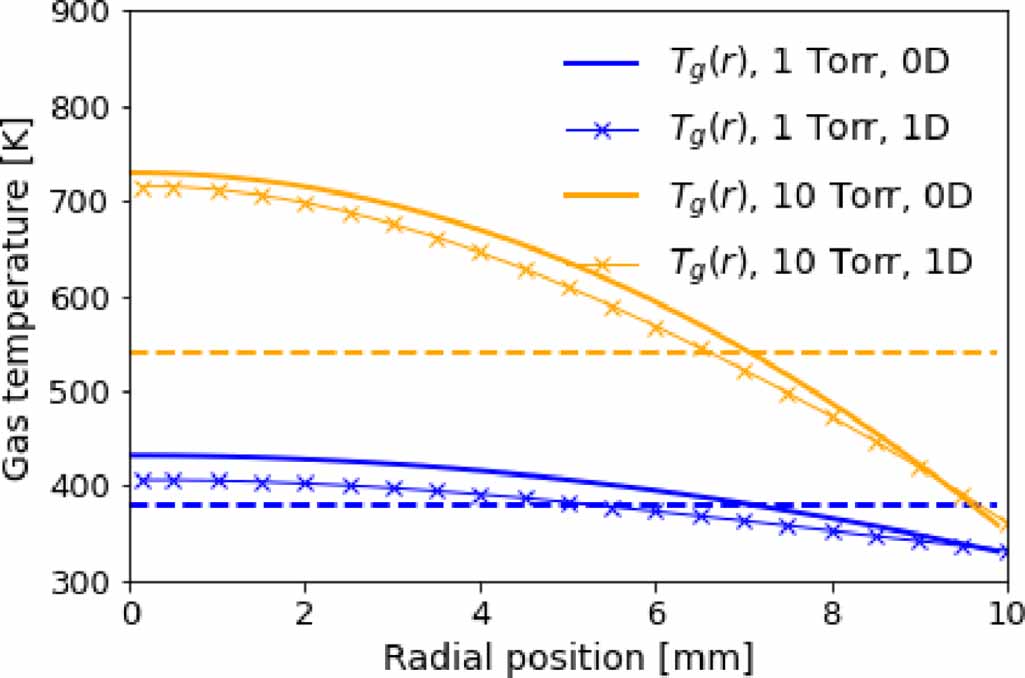
The benchmarking of the 0D model starts by verifying that the radial profiles of the main physical quantities assumed in the 0D model match those obtained in 1D for the conditions under study. One of the main parameters determining the physics in the glow discharge is the translational temperature of neutral atoms and molecules $T_\mathrm{g}$, also called gas temperature. This is assumed in the 0D formulation to follow a parabolic profile (equation (17)). Figure 1 shows that this assumption is valid for a lower-pressure case (1 Torr) and for a higher-pressure case (10 Torr). This figure represents $T_\mathrm{g}(r)$ obtained from the 1D simulation results and from the 0D assumption, that uses $T_\mathrm{g,av}$ (also represented in figure 1) and $T_\mathrm{nw}$ calculated by LoKI.

Zoom In Zoom Out Reset image size

It can be noticed in figure 1 that the 1D result of $T_\mathrm{g}(r)$, resulting from the 1D resolution of the heat equation, stands slightly below the 0D profile and is slightly flatter. However, the difference is lower than 10% and the 1D profile is very close to a parabola. Another feature that can be noticed is that $T_\mathrm{g}(r)$ is more centre-peaked (concave) for higher pressure, with a larger difference between $T_\mathrm{nw}$ and the peak T₀. This is determined by the increased collisionality with pressure (higher $Q_\mathrm{in}$ in equation (18)) that increases $T_\mathrm{g,av}$ and T₀, while $T_\mathrm{nw}$ is kept low due to wall cooling and finite thermal conductivity. Finally, it should be taken into account that, even though the 0D model assumes a parabola, only the average value $T_\mathrm{g,av}$ is actually used in rate coefficient calculations for volume reactions. Therefore, gas heating appears here as a dominant cause of radial gradients that are not fully described in the 0D model and increase with pressure. It could be more accurate for 0D models to consider the whole parabolic evolution of $T_\mathrm{g}(r)$ in the calculation of average rate coefficients (see also equation (34)). However, it is shown in this work that the use of $T_\mathrm{g,av}$ provides reasonable agreement with 1D simulations, which has not been significantly improved by a preliminary implementation of the alternative approach.

The profile of $T_\mathrm{g}(r)$ is directly related to that of the gas density $n_\mathrm{g}(r)$ via the ideal gas law. As such, it is determinant also for the main parameter accelerating electrons and determining electron impact rate coefficients, which is $E/n_\mathrm{g}(r)$. If the axial electric field magnitude E is assumed to be radially uniform and $T_\mathrm{g}(r)$ is assumed to be parabolic, then $E/n_\mathrm{g}(r)$ should also follow a parabolic profile. This assumption is verified in figure 2, for the same pressures studied in the previous figure, by comparing the assumed parabolic profiles of the 0D model with the 1D simulation results. Once more, the 1D radial profiles match closely the parabolic assumption and a more centre-peaked profile of $E/n_\mathrm{g}(r)$ is noticeable for higher pressure. Moreover, it should be noticed again that the average value $E/n_\mathrm{g,av}$ is used to compute average rate coefficients in the 0D model, and not the parabolic profile $E/n_\mathrm{g}(r)$.

Zoom In Zoom Out Reset image size

Another main discharge parameter is the electron density $n_\mathrm{e}$. In homogeneous low pressure cylindrical electropositive discharges where charged particle balance is controlled by electron impact ionization and ambipolar diffusion, $n_\mathrm{e}$ follows a zero-order Bessel function of the first kind, with zero at the cylinder wall (Schottky 1924, Parker 1963, Ikegami 1968, Durandet et al 1989, Fridman and Kennedy 2004, Lieberman and Lichtenberg 2005, Moisan and Pelletier 2012). This implies that the non uniformity of particle loss processes such as wall losses is a second factor inducing radial gradients in the plasma. The presence of negative ions induces a deviation from the Bessel profile (Gousset et al 1989, Guerra and Loureiro 1999, Dias et al 2023). In this work, for the sake of simplicity, we test the 1D simulation results against a Bessel assumption in figure 3. While the agreement is good for the 1 Torr case, it is degraded with pressure, and relative differences of 17% can be observed for the peak value of $n_\mathrm{e}(r)$ at 10 Torr.

Zoom In Zoom Out Reset image size

The increasing deviation of $n_\mathrm{e}(r)$ from the Bessel profile with a change in plasma parameters (pressure, current) can be caused by the development of instabilities. The fact that $T_\mathrm{g}(r)$, $E/n_\mathrm{g}(r)$, $n_\mathrm{e}(r)$ and other species densities all have centred profiles can produce non-linear effects whose intensity increases with pressure leading to discharge stratification and further contraction. The radial contraction of plasmas has been reported in many works (Kenty 1962, Petrov and Ferreira 1999, Kabouzi et al 2002, Dyatko et al 2008, Shkurenkov et al 2009, Golubovskii et al 2011, Wolf et al 2019, Viegas et al 2020, 2021, Vialetto et al 2022). The narrowing of the $n_\mathrm{e}$ profile observed in figure 3 is not due to a departure from the ionization-diffusion regime, since in the current conditions and considering the chosen reaction scheme, diffusive losses are still the dominant charge loss process. In addition, we emphasize once more that all the studied discharge regimes in the present paper correspond to experimental conditions with a visible uniform radial discharge distribution, without striations (Booth et al 2019, 2020, 2022). Furthermore, the contraction is not caused by electronegativity, since according to the 1D simulation results, an increase of attachment in the centre of the plasma, on its own, leads to a flattening of $n_\mathrm{e}(r)$ instead of a contraction. We attribute the pressure-driven change of $n_\mathrm{e}$ radial profile in the positive column of the oxygen glow discharge to inhomogeneous gas temperature, which can lead to the so-called thermal-ionization instability with increasing pressure and current, as in other studies of plasma contraction (Martinez et al 2004, Moisan and Pelletier 2012, Shneider et al 2012, 2014, Ridenti et al 2018, Zhong et al 2019). Indeed, we have observed in figure 2 that $E/n_\mathrm{g}(r)$ is centre-peaked and therefore the electron impact ionization rate coefficient $k_\mathrm{i}$ ($k_\mathrm{i} = {\mathrm{[O_2]} \over n_\mathrm{g}} k_{\mathrm{O}_2 \rightarrow \mathrm{O}_2^+} + {\mathrm{[O]} \over n_\mathrm{g}} k_{\mathrm{O \rightarrow O^+}}$) also has a centre-peaked profile. As a result, the assumption of radial homogeneity leading to a Bessel $n_\mathrm{e}(r)$ profile is not generally satisfied. For the lower-pressure case of 1 Torr, the deviation of $E/n_\mathrm{g}(r)$ from uniformity is small ($E/n_\mathrm{g}$ varies only between 53 and 65 Td in the 1D simulation results) and hence the $n_\mathrm{e}(r)$ profile is very close to a Bessel profile. Nevertheless, the inhomogeneous gas temperature observed in figure 1 increases with pressure and leads to a sharper gradient of $E/n_\mathrm{g}(r)$ at 10 Torr, with values from the 1D results in figure 2 varying between 26 and 51 Td. Indeed, according to the 1D simulation results, while at 1 Torr $k_\mathrm{i}$ varies only between around $2.4 \times 10^{-18}$ m$^3\,\,\cdot$ s⁻¹ at r = 0 and $5.4 \times 10^{-19}$ m$^3\,\,\cdot$ s⁻¹ at r = R, at 10 Torr the variation is much wider, between around $2.3 \times 10^{-19}$ m$^3\,\,\cdot$ s⁻¹ and $8.6 \times 10^{-23}$ m$^3\,\,\cdot$ s⁻¹. It should be noticed that the increased ionization in the plasma core with respect to the plasma edges contributes to increased $T_\mathrm{g}$ in the core via Joule heating, thus forming a self-reinforcing cycle between heating and ionization, that can finally lead to the radial contraction (Zhong et al 2019). The radial contraction cannot be captured by the 0D model, that always considers $n_\mathrm{e,av}$, based on the low radial variation of $n_\mathrm{e}(r)$ under the Bessel assumption.

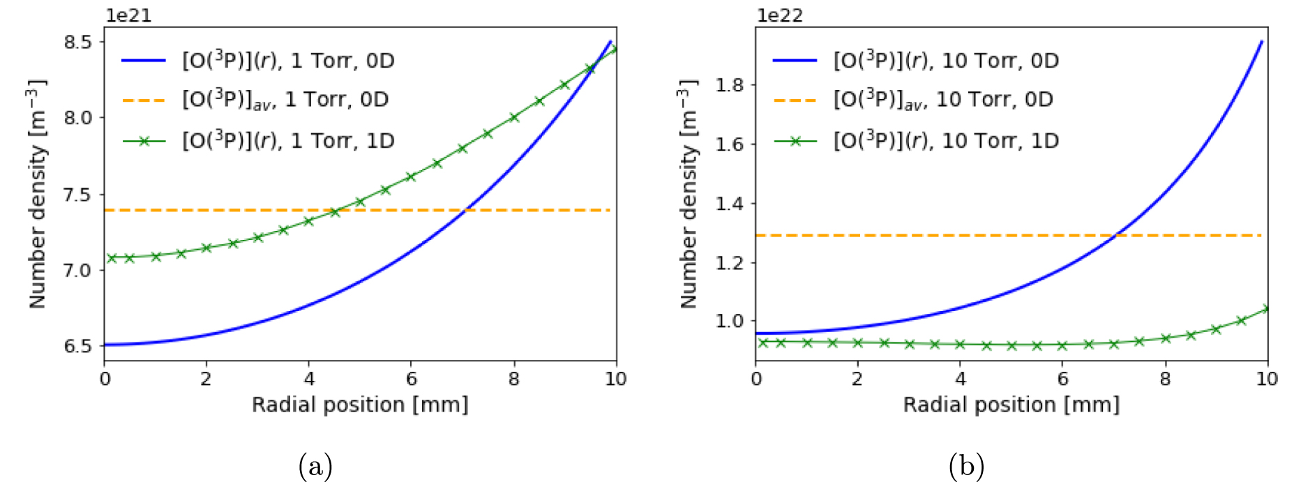
In the study of oxygen glow discharges, the spatial distribution of the number density of atomic oxygen is also of paramount importance, due to the high reactivity of this species. The radial profiles of O(³P) density are represented in figure 4, for 1 Torr (figure 4(a)) and for 10 Torr (figure 4(b)). The 1D simulation result is presented, together with the 0D-calculated average density and the profile obtained from it by assuming proportionality with the total gas density, which, according to the ideal gas law, gives: [O(³P)](r) = [O(³P)]$_\mathrm{av} \times T_\mathrm{g,av}/T_\mathrm{g}(r)$). This assumption is based on an assumed radial uniformity of source (electron-impact dissociation) and loss (diffusion and recombination at the surface and in volume) processes of atomic oxygen, consistent with $\gamma_{j} \ll 1$ (see tables 1 and 2) in equation (16).

Zoom In Zoom Out Reset image size

Figure 4 shows that, for both pressures, the 1D and 0D models provide O(³P) densities within the same order of magnitude but with slightly different spatial evolutions. For 1 Torr, the 1D simulation result approximately follows the ideal gas law, that provides a difference between minimum and maximum values below a factor 2. The 0D parabolic profile provides a good agreement near the wall but slightly lower values in the bulk of the plasma. However, for 10 Torr, the 0D parabolic profile provides a similar result to 1D in the bulk but a factor 2 higher near the wall. Indeed, at 10 Torr, the 1D radial profile of O(³P) density is almost flat, rather than parabolic. The reasons for not following the ideal gas law are related with diffusivity, O atom wall losses and the radial non-uniformity of $E/n_\mathrm{g}(r)$ (see figure 2) and thus of the electron impact dissociation rate coefficient. It has been shown in Booth et al (2019) that oxygen atoms in a similar DC discharge conditions are predominantly lost by recombination on the tube surface and hence the assumption of radially uniform losses is not fulfilled.

As a result of the previous analysis, we consider that, when using a 0D model without access to the resolved spatial distribution of O(³P) density, it is generally more accurate to consider flat profiles than parabolic ones. This consideration has implications on the calculation of source and loss terms in the rate balance equations (equation (12)) and on the calculation of wall loss probabilities from wall loss frequency measurements (equation (5)) by considering [O(³P)]$_\mathrm{nw}$ = [O(³P)]$_\mathrm{av}$.

In this section, it has been shown that the radial profiles of some of the main discharge parameters obtained through 1D simulation results in the studied conditions are not far from those assumed in 0D models: $T_\mathrm{g}(r)$ and $E/n_\mathrm{g}(r)$ are approximately parabolic, $n_\mathrm{e}(r)$ are near-Bessel and [O(³P)](r) are almost flat. The deviation from these assumptions generally increases with pressure, due to the pressure-driven narrowing of radial profiles, but is still rather small (below a factor 2) up to 10 Torr in the positive column of oxygen glow discharges. This shows that, even though the 1D model takes the full radially-resolved profiles and the 0D model uses only averaged quantities, it is valid to compare the averaged values from both models, as they refer to the same type of radial profiles. That type of comparison is the subject of the next section.

To proceed with the benchmarking, $T_\mathrm{g,av}$, $T_\mathrm{nw}$ and the average values of $E/n_\mathrm{g}$ are compared between the 0D and 1D simulation results for the whole range of pressures between 0.5 Torr and 10 Torr, in figure 5. It can be noticed that all the values are very close, with differences below 5%. $T_\mathrm{g,av}$ obtained from the 1D model is always slightly lower than the one from the 0D calculations, while $T_\mathrm{nw}$ is slightly higher in the 1D simulations, which reflects the flatter radial profiles of $T_\mathrm{g}(r)$ in 1D results observed in figure 1. $E/n_\mathrm{g}(p)$ follows the same evolution with pressure in both models, with maxima below 75 Td at 0.5 Torr and minima above 35 Td at 10 Torr. The electron temperature $T_\mathrm{e}(p)$ (not represented here) presents a similar profile, with maxima at around 2.7 eV and minima near 2.1 eV.

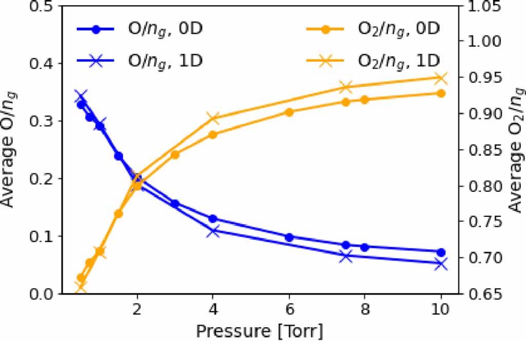
Zoom In Zoom Out Reset image size

The comparison proceeds with the dissociation degree. Figure 6 shows the average molar fractions of O and O₂ for the several pressures. The calculation of the molar fractions includes all the O and O₂ neutral and ionized species considered in the models. The agreement between 0D and 1D models is good but decreases with pressure. Indeed, at higher pressures, the plasma is slightly (a few percent) more dissociated in the 0D model than in the 1D case, as already suggested by the results in figure 4. This small difference is justified mostly by the particle balance of O(³P), where electron impact dissociation of O₂(X) and O₂(a) are the main source terms, and volume and wall recombination are the main loss terms. As the $E/n_\mathrm{g}$ profile is centre-peaked and the O(³P), O₂(X) and O₂(a) profiles are convex (lower in the centre and higher on the edges) in the 1D simulation results at 10 Torr (see figures 2, 4 and 10), dissociation is hindered and recombination is promoted, relatively to the 0D results that only consider average values in rate calculations.

Zoom In Zoom Out Reset image size

The reasonable agreement between 0D and 1D simulation results is also observed when analysing the average number densities of charged species. Figure 7(a) shows only the main charged species: electrons, O⁻ and O$_2^+$; since the densities of the remaining ions (O$_2^-$, O$_3^-$, O⁺ and O$_4^+$) are negligible. While the average electron density always presents a good agreement between 0D and 1D simulation results, the plasma contains more (up to 25%) negative and positive ion densities in the 1D model than in 0D. The difference increases with pressure and is attributed to the centre-peaked profiles of $n_\mathrm{e}$ and $E/n_\mathrm{g}$ (see figures 2 and 3) that promote the production of negative and positive ions via electron impact reactions (attachment and ionization) in 1D simulations with respect to the 0D model, that considers only averages. Concerning the destruction of O⁻ and O$_2^+$, it takes place mostly via detachment by collisions with species with convex (lower in the centre and higher on the edges) radial profiles (O⁻ case) and via wall recombination (O$_2^+$ case). As these species have centre-peaked radial profiles (see figure 7(b)), their destruction is relatively decreased in 1D, which also contributes to the observed higher average densities.

Zoom In Zoom Out Reset image size

Concerning excited state average densities, these are represented from 0D and 1D simulation results in figures 8 and 9. Despite the logarithmic vertical scale in the figures, it can be noticed that the agreement between the two models is quite good for most species. However, there is significantly more (a factor 3 at 10 Torr) O₃ average density in the 1D simulation results than in the 0D case. The deviation increases with pressure. It is important to assess this difference.

Zoom In Zoom Out Reset image size

Zoom In Zoom Out Reset image size

The main reactions of production of O₃ at the higher pressures, e.g. 10 Torr, and their rate coefficients (Braginskiy et al 2005) are:

$$\begin{align} & \mathrm{O\left(^3P\right) + O_2(X) + O_2(X) \rightarrow O_3 + O_2(X)}, \end{align} \tag{ 22 }$$

$$\begin{align} & k_\mathrm{O\left(^3P\right) + 2 O_2(X)} = 5.6 \times 10^{-41} \times T_\mathrm{g}^{-2} \ \mathrm{m^6}\,\,\, {\cdot}\,\,\, \mathrm{s^{-1}}, \end{align} \tag{ 23 }$$

$$\begin{align} & \mathrm{O^- + O_2(a) \rightarrow e + O_3}, \end{align} \tag{ 24 }$$

$$\begin{align} & k_\mathrm{O^- + O_2(a)} = 1.9 \times 10^{-16} \ \mathrm{m^3}\,\,\, {\cdot}\,\,\, \mathrm{s^{-1}}, \end{align} \tag{ 25 }$$

$$\begin{align} & \mathrm{O_2(X) + O\left(^3P\right) + O\left(^3P\right) \rightarrow O_3 + O\left(^3P\right)}, \end{align} \tag{ 26 }$$

$$\begin{align} & k_\mathrm{O_2(X) + 2 O\left(^3P\right)} = 2.15 \times 10^{-46} \times \exp{(345 \ \mathrm{K}/T_\mathrm{g})} \ \mathrm{m^6}\,\,\, {\cdot}\,\,\, \mathrm{s^{-1}}, \end{align} \tag{ 27 }$$

where $k_\mathrm{O\left(^3P\right) + 2 O_2(X)}$, $k_\mathrm{O^- + O_2(a)}$ and $k_\mathrm{O_2(X) + 2 O\left(^3P\right)}$ are respectively obtained from Rawlins et al (1987), Belostotsky et al (2005)and Steinfeld et al (1987).

On average, the 1D results at 10 Torr contain slightly more O⁻ and O₂(X) than the 0D results, which promotes ozone production. Conversely, the 1D results contain slightly less O₂(a) and O(³P) averaged densities, which hinders ozone production. Therefore, an analysis of the average densities of reactants is inconclusive in terms of justifying the O₃ density difference. Nevertheless, we should notice that the rate coefficients for O₃ production decrease with $T_\mathrm{g}$. Despite similar $T_\mathrm{g,av}$, $T_\mathrm{g}$ is lower on the edges in the 1D model than in 0D, where only $T_\mathrm{g,av}$ is used (see figure 1). This is also the region where the reactants have higher number densities, as is shown in figure 10, where 1D radial profiles are compared with the averages used in the 0D model at 10 Torr. Together, these two factors determine higher source of O₃ in the 1D model than in 0D.

Moreover, regarding the losses of O₃, we should notice that at 10 Torr the main reactions of destruction of O₃ and their rate coefficients (Braginskiy et al 2005) are:

$$\begin{align} & \mathrm{O_2(a) + O_3 \rightarrow O\left(^3P\right) + O_2(X) + O_2(X)}, \end{align} \tag{ 28 }$$

$$\begin{align} & k_\mathrm{O_2(a) + O_3} = 5.2 \times 10^{-17} \times \exp{(-2840 \ \mathrm{K}/T_\mathrm{g})} \ \mathrm{m^3}\,\,\, {\cdot}\,\,\, \mathrm{s^{-1}}, \end{align} \tag{ 29 }$$

$$\begin{align} & \mathrm{O_2(b) + O_3 \rightarrow O\left(^3P\right) + O_2(X) + O_2(X)}, \end{align} \tag{ 30 }$$

$$\begin{align} & k_\mathrm{O_2(b) + O_3} = 1.5 \times 10^{-17} \ \mathrm{m^3}\,\,\, {\cdot}\,\,\, \mathrm{s^{-1}}, \end{align} \tag{ 31 }$$

$$\begin{align} & \mathrm{O\left(^3P\right) + O_3 \rightarrow O_2(X) + O_2(X)}, \end{align} \tag{ 32 }$$

$$\begin{align} & k_\mathrm{O\left(^3P\right) + O_3} = 7.68 \times 10^{-18} \times \exp{(-2060 \ \mathrm{K}/T_\mathrm{g})} \ \mathrm{m^3}\,\,\, {\cdot}\,\,\, \mathrm{s^{-1}}, \end{align} \tag{ 33 }$$

where $k_\mathrm{O_2(a) + O_3}$ and $k_\mathrm{O\left(^3P\right) + O_3}$ are obtained from Baulch et al (1984) and $k_\mathrm{O_2(b) + O_3}$ comes from Slanger and Black (1984).

The reactants for these loss processes (except O₃ itself), O₂(a), O₂(b) and O(³P), have slightly lower average densities at high pressures in the 1D simulation results than in the 0D case (see figures 8 and 9). Furthermore, the rate coefficients for O₃ destruction increase with $T_\mathrm{g}$, and thus are lower in the plasma edges, where most reactants, O₂(a), O(³P) and especially O₃, have higher densities (see figure 10). These two factors contribute to a relatively lower destruction of O₃ in the 1D model. We can conclude that the subtle differences in $T_\mathrm{g}$ and species densities induced by dimensionality lead to both higher production and relatively lower destruction of O₃ in the 1D model than in the 0D case. The difference could potentially be decreased by using parabolic profiles of $T_\mathrm{g}(r)$, $n_\mathrm{g}(r)$ and $E/n_\mathrm{g}(r)$ and Bessel profiles of $n_\mathrm{e}(r)$ in the 0D model rate coefficient calculations, instead of average values. As an example, this means calculating electron-O₂(X) reaction rate coefficients $k_\mathrm{av}$ as:

$$\begin{align} k_\mathrm{av}={\int_0^R n_\mathrm{O_2(X)}(r) \ n_\mathrm{e}(r) \ k(T_\mathrm{g}(r),E/n_\mathrm{g}(r)) 2 \pi r \mathrm{d}r \over n_\mathrm{O_2(X),av} \ n_\mathrm{e,av} \int_0^R 2 \pi r \mathrm{d}r}, \end{align} \tag{ 34 }$$

instead of $k_\mathrm{av} = k(T_\mathrm{g,av},E/n_\mathrm{g,av})$. However, as can be seen in figure 10, some species densities do not follow the parabolic $n_\mathrm{g}(r)$ profile. A preliminary implementation of this approach has shown no significant improvements on the agreement with 1D results.

The differences found between 0D and 1D averaged simulation results are summarized in figure 11. This figure represents, as a function of pressure, the relative differences between the values found for temperatures ($T_\mathrm{g}$, $T_\mathrm{nw}$ and $T_\mathrm{e}$), reduced electric field ($E/n_\mathrm{g}$) and species densities. Concerning species densities, the averages of the relative differences of all charged species densities and all neutral species densities are considered (i.e. the relative differences are summed and the sum is divided by the number of species in question).

Zoom In Zoom Out Reset image size

Zoom In Zoom Out Reset image size

Figure 11 shows that, in the whole pressure range between 0.5 Torr and 10 Torr, there is a very good agreement (with differences below 5%) on average temperatures and reduced electric field obtained from 0D and 1D models. The disagreement on average species densities is also relatively low, but it increases with pressure. Indeed, the relative differences lie below 20% at 1 Torr and between 50% and 60% at 10 Torr. The fundamental reason for this increase appears to be the pressure-driven narrowing of radial profiles. As pressure increases, radial profiles become more centre-peaked and radial gradients become sharper in the 1D description. As a result, the success of 0D models in describing oxygen glow discharges through volume averaged quantities decreases with pressure. In the case under study, with 1 cm tube inner radius, in light of the results, we would recommend the use of 0D global models to describe this plasma in the pressure range up to 10 Torr, but not above, since the deviation with respect to radially-resolved results is expected to increase.

Different tube radii of 0.5 cm and 2 cm have been used for this study for a few pressure values. This has been done both keeping I = 30 mA, thus changing the current density, and keeping the average current density, thus changing I. It has been found that the upper limit of pressure of validity of global models to describe the positive column of oxygen glow discharges is mostly independent of the tube radius, within the R limits considered ($R = 0.5 - 2$ cm).